
Basics
The task of strength of materials is to determine which external forces a solid body can withstand (for example, a structure, a structural member, or soil). To answer this question, two criteria are used: on the one hand, stresses must not exceed certain limits that depend on the type of material, and on the other hand, the balance between external and internal forces must be stable. Accordingly, all problems in strength of materials can be divided into “stress problems” and “stability problems.”
For bars and beams and the members composed of them (trusses, frames), stress determination is carried out in two steps: first, based on the applied external forces, the resultant of the internal forces transmitted through the cross-section is calculated, and then the stresses are determined from these “section forces.” The first part of the procedure is a separate, extensive discipline, structural statics, which has its own developed methods and is usually separated from strength of materials, whose task is reduced to determining stresses from the given section forces.
Basic concepts of material strength
The definition of stress is reached through the following basic considerations. Let there be an equilibrium system of external forces acting on a body. Suppose that we have divided the body by an arbitrary cross-section into two parts, and that we have removed one of them together with the forces acting on it; then its action on the other part, in order for the force balance and the distribution of deformations to remain unchanged, must be replaced by additional forces transmitted through the cross-sectional area. These “internal” forces are continuously distributed over the cross-sectional area, so that each area element dF corresponds to a force dβ. If the quotient dβ dF is formed and the limiting transition dF -> 0 is made, then this quotient approaches the limiting value called stress. The stress in a given surface element is, like dβ, and can be decomposed into components normal and tangential to dF, the normal stress σ and shear stress τ.
If sections are drawn through the same point in different directions, different stresses will correspond to them as well. In particular, if an elemental cuboid, shown in fig. 1, is isolated from the body, a stress vector will act on each of its six faces, which can be decomposed into three components in the directions of the coordinate axes x, y and z. The stresses acting on opposite faces differ from one another only by a differential, of course, so it is necessary to distinguish 3 * 3 = 9 component stresses, which are designated as follows:
Normal stresses σ are assigned the index of the axis along whose direction they act and are considered positive if they cause tension, negative if they cause compression. Shear stresses τ are given two indices, the first of which is the same as the index of the corresponding normal stress, and the second refers to the axis in the direction of which the shear stress acts. If the positive direction of the corresponding normal stress is in the direction of the positive (negative) coordinate axis, the shear stress is also considered positive if it acts in the direction of the positive (negative) coordinate axis.
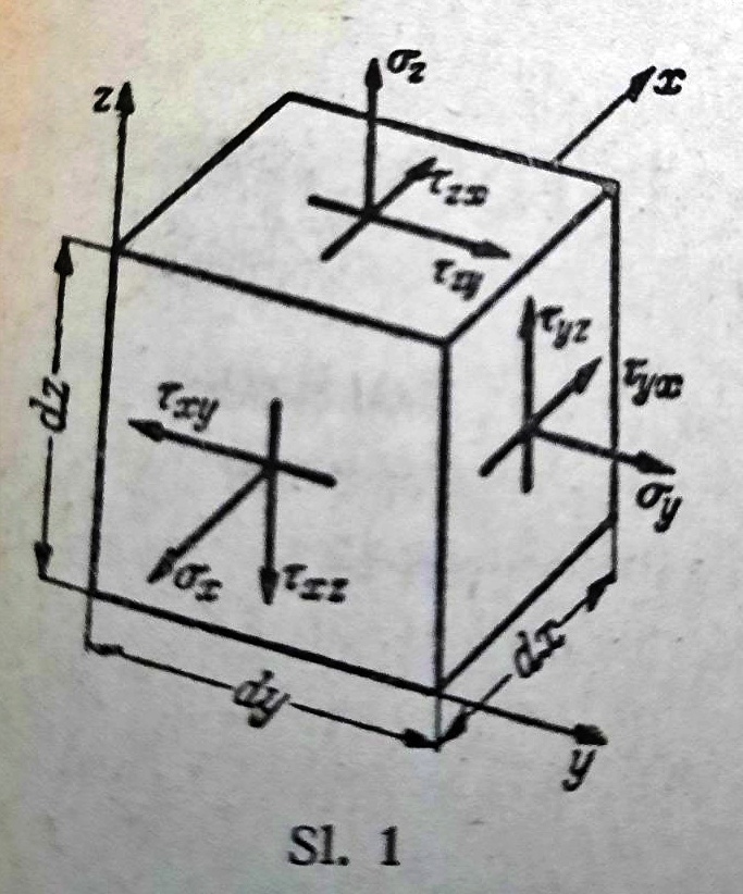
Figure 1.
Conjugacy of shear stresses
If, for the elemental block, fig. 1, the condition is set that the moment of all forces with respect to the x-axis is zero, one obtains τyz dx dz * dy = τzy dx dy * dz From this, and from the two corresponding equations for the y and z axes, it follows that shear stresses with the same indices are equal to one another τxy = τyx, τyz = τzy, τzx = τxz (1)
Component deformations
That the stresses defined above have physical meaning follows from their relation to the deformation undergone by every body under the influence of external forces. Fig. 2 shows an elementary cuboid that before deformation was rectangular and had edge lengths dx, dy, dz. The edge lengths after deformation can be denoted as dx + Δdx, dy + Δdy, dz + Δdz; the ratios εx = Δdx|dx, εy = Δdy|dy, εz = Δdz|dz are called strains. These are dimensionless quantities and, for all materials relevant in construction, are small compared with 1. In addition to elongation of the edges, the elementary cuboid dx * dy * dz may also undergo a change in the originally right angles between its faces.
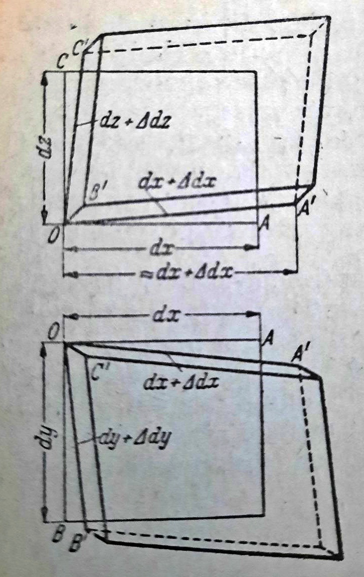
Figure 2. component strain
Let, after deformation, the angle between the planes meeting along edge OC be equal to 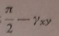 , and likewise let the reduction of the right angle along edge AO be equal to γyz, and the reduction along edge OB be equal to γzx. These three changes of angle γxy, γyz, γzx are called shear strains and are also always small compared with 1. With the six component ε and γ, the deformation of the elementary hexahedron, “small deformation,” is completely determined. The change in the volume element d_V = dx * dy * dz_ is ΔdV = (dx + Δdx) (dy + Δdy) (dz + Δdz) - dx dy dz, from which, when products of strains are neglected as small quantities of higher order, the volumetric strain ϱ = ΔdV|dV = εx, εy, εz (2) is obtained
Shifts
The deformation of a solid body can also be described completely by assigning to each of its points the displacement that point has undergone. If finite displacements corresponding to rigid-body motion are excluded from consideration by adopting, if necessary, a movable coordinate system in the calculation, then the component displacements μ, ν, ω are always small quantities, and their derivatives with respect to the coordinates are small compared to 1. Under that assumption, according to fig. 3 the length of the linear element OA = dx after deformation

therefore  (3)
(3)
Similarly, from fig. 3 it can be seen that the shear γxy γ1 + γ2: and also
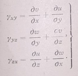 (4)
(4)
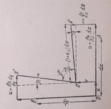
Figure 3 slip
 (5)
(5)  (6)
(6)
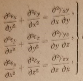
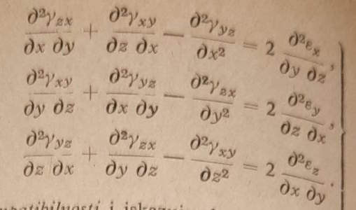
These relations are called compatibility conditions and state that the deformed elements can fit together like a mosaic so that the space is continuously filled, which cannot be achieved if the deformations of the elements are arbitrary. The compatibility conditions are differential equations, so, of course, all six component strains for each individual block are mutually independent, but their arrangement in any finite spread region is governed by the conditions (5) and (6).
Since these conditions are obtained by differentiation from equations (3) and (4), part of the constraints contained in the original equations is lost in their derivation. Therefore, it is not sufficient for only one of these two systems of equations to be satisfied; both systems of equations must be satisfied if deformation compatibility is to be ensured.
Differential equations of the elasticity system
The following equations are used to calculate stresses and strains in elastic bodies:
Equilibrium conditions of the volume element. The conditions that the moments about the three axes are equal to zero were already used in deriving equation (1). The force equilibrium conditions are given according to fig. 4
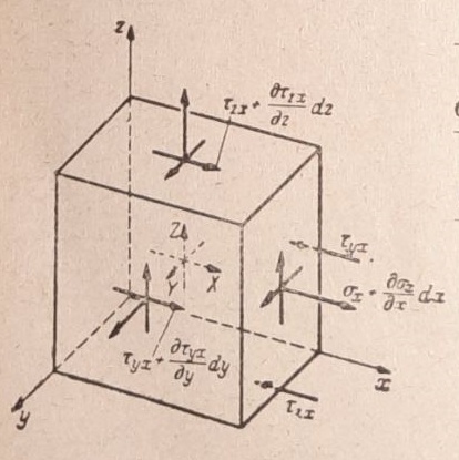
Figure 4
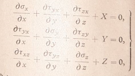
(7a-c)
If X, Y, Z denote the components of body forces (e.g. weight, centrifugal force) per unit volume. Relations between stresses and strains. This means the relationship between stress components and strain components. In elasticity theory, as a rule only a linear relationship is considered, expressed by Hooke’s law:
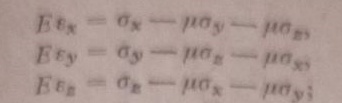
(8a-c)

(8d-f)
If equations (8a-c) are solved for stresses, one obtains

(8 a)
and two corresponding equations. Hooke’s law expressed by equation (8) does not represent a strictly fulfilled natural law, but an idealization of actual behavior, which departs from it more or less, depending on the material and the magnitude of the stress. Given that the mathematical treatment of material strength problems with complicated, nonlinear relationships between stresses and strains causes incomparably greater difficulties and can in fact be carried out only in the simplest cases, even for those materials (concrete!) whose behavior departs significantly from Hooke’s law, calculations based on it must be used as the first, and mostly the only approximate solution, which is in any case usually very useful and provides insight that is more than merely qualitative. G = E|2 (1+μ).
It necessarily follows from the relation between stress and strain (8), from the transformation equations (16) for stresses, and from the corresponding system of equations for the component strains. E and G have the dimension of stress and, for all construction materials, are large compared with the stresses σ and τ that may occur. This fact underlies the assumption adopted everywhere in elasticity theory that deformations are small. The coefficient of lateral expansion (Poisson’s ratio) μ is dimensionless and is always between 0 and 1/2.
Relationships between component strains and displacements. These relationships are given by equations (3), (4). They are of a purely geometric nature. These three systems give 3+6+6=15 equations for 15 unknowns, i.e. for 6 component stresses, 6 component strains and 3 component displacements. They are therefore sufficient to determine these unknowns. The mathematical treatment of such an extensive system of differential equations is, of course, possible only in special cases. If in equation (8) the component strains are replaced by the component displacements according to equations (3) and (4), and then the normal stresses σ and shear stresses τ, according to equations (8 d - f), are introduced into the equilibrium conditions, equation (7), differential equations are obtained which are called the fundamental equations of the theory of elasticity.
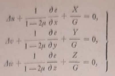
(9)
where 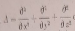 denotes the Laplace operator. In view of (2), these are three differential equations with three component displacements μ, ν, ω; from these, by differentiation on the basis of (3), (4) and (8), all component stresses and strains can be obtained. Equations (9) often represent a convenient starting point for studying special cases.
Deformation work
Definition
When a beam is loaded, the points of application of the external forces undergo elastic displacements and the forces thereby perform a certain amount of work. In this way, the energy supplied can be transformed into different forms. If the loading is applied suddenly, so that the deformation process has a considerable speed, part of this energy is transformed into kinetic energy, which dissipates over time, either by being transmitted to the ground as an elastic wave that disappears into infinity, or by being converted into heat through internal friction. If the loads are applied so gently that no noticeable increase in kinetic energy occurs, that is, if the gradually increasing loads starting from zero are in constant equilibrium with the internal forces, the energy is evidently spent exclusively on deforming the body and is then called deformation work.
We will first demonstrate the calculation of deformation work on a part loaded in uniaxial tension (fig. 5).
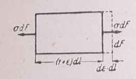
Let the existing stress σ and the corresponding strain ε undergo increments dσ and dε. Then the force σdF over the path dε * dl will perform work σdF * dεdl = σdεdV, if dV denotes the volume of the small element. If the stress increases from zero to its final value and the strain accordingly from 0 to ε, the total work performed per unit volume will be:
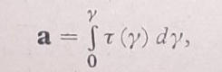
Similarly, for an element loaded by shear stress τ (fig. 6), the deformation work per unit volume (specific deformation work, elastic potential):
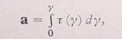
where only one of the four forces τ * dF does work.
In the general case, when all six stress components act on an elemental portion, the specific deformation work is obtained by summing the work of the individual stress components:
(10)
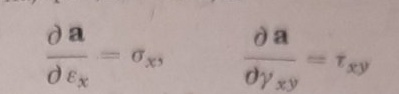
By differentiating with respect to the upper limit of each of these integrals, relations are obtained that hold in the most general case:
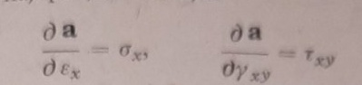
(11)
and similarly for the other component deformations. If the body is elastic, every specific state of stress corresponds to exactly the same state of deformation, regardless of whether the state is reached during loading or unloading. Then the integrals contain single-valued functions, and the total energy expended during loading and then complete unloading is a = 0, since in this case the upper limits of the integrals become zero. Therefore, the total energy supplied to the body during loading is recovered during unloading.
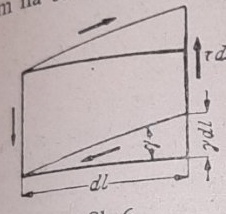
Figure 6
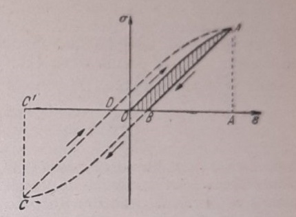
Figure 7
For a partially elastic body, the relation between stress and deformation for the entire loading and unloading cycle has the form approximately shown in fig. 7 by the lines O A B. The energy  supplied during loading is equal to the area OAA, and the energy returned during unloading to the area ABA, so that the work corresponding to the shaded area is lost (converted into heat). If, in an oscillatory process, the stress changes periodically between the positive limiting value
 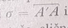 and the negative limiting value,
 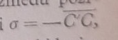 the inelastic deformation proceeds similarly to that shown by the dashed lines in fig. 7 and during each oscillation period the energy DABCD is converted into heat per unit volume. Such behavior during deformation, in which deformation lags behind stress, is called elastic hysteresis, and the curve DABCD is the hysteresis loop.
Deformation work and Hooke’s law
If Hooke’s law is introduced into the integrals in equation (10), integration can be performed, and the following expressions are obtained for the specific strain energy:

(12a)
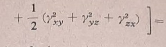
(12b)
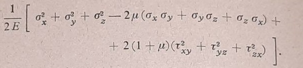
(12c)
If the second of these forms is substituted into equation (11), Hooke’s law is obtained again, equations (8), in the form solved for stresses. The statement that the deformation work depends on the component deformations, as shown by equation (12b), is therefore equivalent to Hooke’s law. When equation (12c) is differentiated with respect to the stresses, one obtains

(13)
These forms, unlike the forms (11), are valid only for bodies that behave according to Hooke’s law and cannot be applied when the relationships between stresses and strains are different. It is understood that only the component strains caused by stresses are on the right-hand side of equations (13), while all others that may have arisen due to temperature change, creep, swelling, recrystallization, etc. are excluded.
INTEGRAL CONCEPTS IN THE THEORY OF ELASTICITY
Virtual displacements. Principle of minimum potential energy
Just as Hooke’s law, equations (8), can be replaced by a single equation (12b), so too the principle of virtual displacements may be introduced instead of the equilibrium conditions, as a generally valid fundamental law of mechanics. This law states that equilibrium states are characterized by the fact that the total work performed by all forces during a small change in the deformation state is equal to zero. If the small changes in elastic displacements are denoted by δμ δν, δω, then the volume forces defined by equation (7) perform virtual work

and the surface forces px, py, pz acting on the element dF of the outer surface of the body work 
where the triple integral refers to the entire volume, and the double integral to the entire outer surface of the body. To calculate the work done by internal forces, equation (12b) is used, so the work per unit volume is obtained
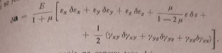
The principle of virtual displacements therefore gives

(14)
If the loads X, Y, Z px, py., pz are understood as components of gravity (self-weight and external load), the integrals on the right-hand side represent the potential energy lost by these loads, while the left-hand side represents the increase in potential (elastic) energy of the body, so this principle states that the total potential energy of the carrier and the loads resting on it in the case of equilibrium has an extreme value. If this extreme value is a minimum, the equilibrium is stable.
The principle of minimum potential energy expressed by equation (14), the expression (12b) for deformation work, and the compatibility conditions of strains (5), (6) represent a system of equations that is sufficient for building the theory of elasticity and is in essence equivalent to the system of equations. This system can be particularly useful in cases where satisfying the differential equations (9) presents computational difficulties and therefore an approximate solution must be sought; for example, for displacements one first assumes a suitable form containing several free constants, and these are then determined from the requirement that equation (14) be satisfied. In this way, one does not obtain a strict solution of the problem, but only the best approximation that can be achieved with the chosen form of the solution. Whether the approximation is sufficient depends primarily on the adopted form of the solution, and successful application of this method therefore requires skill and experience.
Castigliano’s principle
While in the principle of minimum potential energy all deformation states that satisfy the conditions of deformation compatibility are compared and from them those for which the corresponding stresses satisfy the conditions of equilibrium are selected, in Castigliano’s principle all stress states that satisfy the conditions of equilibrium are compared and from them those for which the corresponding deformations satisfy the conditions of deformation compatibility are selected. This principle states: of all possible equilibrium states, the one that actually occurs is the one corresponding to the smallest deformation work. Castigliano’s principle, together with equation (12c) for deformation work and the equilibrium conditions, forms a system of equations sufficient for determining the strength of materials. Since this principle includes Hooke’s law, its applicability is tied to the assumption that deformations can be completely described by this law. This requires not only linear elastic material behavior, but also excludes temperature changes.
Behavior of materials beyond the elastic limits
Phenomena under static loading
Deformation of material under the influence of stress is a very complex phenomenon, so it must be simplified in various ways in order to be understood. One of these simplifications is the assumption that loads are applied gradually, as is done, for example, with specimens during tension and compression tests.
If a steel rod loaded in tension is subjected to a load that increases gradually and its elongation ε is measured, the diagram shown in fig. 8 is obtained. At first the elongation is very small and proportional to the stress, as required by Hooke’s law. From a certain stress onward, proportionality ceases and the elongation increases more rapidly. The exact position of this proportional limit is difficult to determine. The more accurate the measurement, the lower it is found. For most materials it lies at σ = 0, and Hooke’s law then represents only the first approximation to elastic behavior, the first term in the Taylor series expansion of the function ε = ε(σ) in the vicinity of the origin of coordinates.
If the rod is unloaded, it is observed that, when the stress was not too great, the deformation also disappears, in accordance with Hooke’s law. But this also changes if a certain stress is exceeded that lies near the limit of proportionality, the so-called elastic limit; then the total deformation consists of an elastic (recoverable) and an inelastic (permanent) part. The elastic limit also cannot be determined exactly; it lies lower the greater the measurement accuracy. However, since it has great technical significance, because it represents the limit of validity in almost all calculations in strength of materials, and at the same time the limit at which the first permanent damage occurs, for testing samples it is sharply defined by an adopted convention, so, for example, as the 0.2% limit is designated the stress at which the permanent elongation reaches 0.2%.
Immediately after the elastic limit is exceeded, deformation increases sharply and can be observed with the naked eye; under nearly constant stress, the bar continues to elongate. This stress is called the yield point. In hydraulic materials-testing machines, after the onset of yielding, a more or less pronounced drop in stress can also be observed; as indicated in fig. 8 by the dashed curve; then the maximum is called the upper yield point, and the constant yield stress that follows is the lower yield point.
After a certain elongation is reached, which is almost completely inelastic, the stress begins to rise again and the material strain-hardens. In this loading range, a noticeable reduction in the cross-section of the rod occurs due to (inelastic) lateral contraction, and the further course of the stress-strain diagram depends primarily on whether, when calculating the stress σ, the tensile force P acting on the rod is divided by the original cross-section F0 or the current cross-section F. For engineering purposes, the stress P|F0 is of interest. This stress reaches a maximum, which is called the material strength, and once that maximum has been passed, the rod necks down sharply at one point and breaks. The “actual stress” P|F increases until failure.
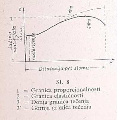
Figure 8.
The behavior of other metals differs in many respects from that described here. Yielding is often not pronounced, and hardening begins immediately after the elastic limit is exceeded. In brittle materials (stone, glass, concrete), inelastic deformations are generally small, and failure occurs even at small elongations. The total elongation a material undergoes up to failure is a measure of the ductility (opposite: brittleness) of the material, and for steel it is precisely specified in the technical requirements. However, since immediately before failure further deformation concentrates in the adjacent necked sections, a different value of elongation at fracture is obtained, depending on whether a larger or smaller part of the bar is taken as the gauge length, so that in order to obtain unambiguous and mutually comparable results, a certain convention must be adopted in advance. Elongation at fracture is usually measured by marking on a round bar of diameter d before the test the gauge length Ι = 10 d and calculating from its elongation ΔΙ the elongation at fracture εs_Ι = ΔΙ|Ι ._ If it is necessary to test bars of a different cross-section, the gauge length is determined according to the diameter of a circular cylindrical bar that has the same cross-sectional area.
Long-term loading
For the tensile test procedure, it is fairly irrelevant whether the load to failure is increased over 10 m minutes or several hours. However, if the load acts for years or decades, under certain conditions it is observed that, even below the yield limit, deformation under constant stress increases slowly over time. The elastic part, i.e. the part that disappears upon complete unloading, does not change noticeably. This increase in inelastic deformation that occurs over a long period of time is called creep. In metals, except lead, creep is significant only at high temperatures; however, for the structural engineer it plays a role in concrete, which yields slightly under compression, so that the stress increases in the compressed reinforcement, if any exists.
Variable load
In order for the mechanical characteristics of a material obtained in a tensile test to be used as a criterion for the allowable loading of structures, it is necessary that the material withstand, under each subsequent loading, the stress it once withstood without damage. This condition is not met if the material is subjected to frequent repeated loading and unloading, as is, for example, the case with beams loaded by the inertial forces of machines that are not fully balanced. By sufficiently frequent repetition of loading, a structural member can be brought to failure even at a stress far below the strength of the material determined by a standard static test. This type of failure is called fatigue failure. The number n of load cycles that a material can withstand depends on the magnitude of the stress σ, so that it is greater the smaller the stress. A typical example of this dependence is shown in Fig. 9, from which it can be seen that for material strength there is a lower limit that it can withstand even with an arbitrarily large number of load cycles, and which is called the dynamic strength of the material. Diagrams of this type (Fig. 9) are called Wöhler curves.
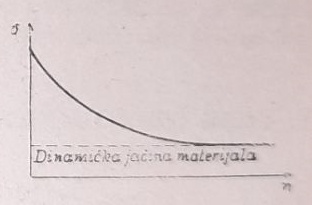
Image 9.
Structural safety
Two limit loads are significant for structures: the load at which the first permanent damage occurs (the yield limit), and the load at which the load-bearing capacity of the structure is exhausted, causing it to fail (the failure limit). Since, at least approximately, the assumptions of mechanics of materials (small displacements, Hooke’s law) apply up to the yield limit, safety against permanent deformation can be reliably assessed in all those cases in which the mathematical difficulties can be overcome. If stress is proportional to load, the ratio of the yield stress to the greatest stress occurring in the structure is equal to the ratio between the load at which yielding occurs and the actual load, and represents the factor of safety against yielding. However, in a number of cases this simple relationship does not exist: bending when tension is excluded, compression between convex surfaces, systems whose structure is variable and, especially unfavorable, bending with an axial force. In all these cases a relatively small increase in load can lead to a large increase in stress, and then it is not sufficient to apply the customary factor of safety to the stresses; it must instead be applied to the load.
The phenomena that occur after the yield limit is exceeded up to failure can in most cases be followed only qualitatively. If the material is ductile, the parts in which the yield limit is reached first, and which then deform further at constant stress or stress that increases only slightly, contribute little to carrying the further load, so that the remaining, less stressed parts of the structure, insofar as this is possible given its structure, take a greater part in bearing the load. In this tendency toward equalizing stress peaks lies a certain reserve of safety, which can be used in calculation if the permanent deformation of individual parts, resulting from only one significant load, is not harmful (limit load method).
If the material is brittle, the first permanent damage appears in cracks, which cause an even greater concentration of stress at the endangered point and immediately trigger failure. Failure due to fatigue, even in ductile materials, has the characteristics of brittle fracture.
Relations between stresses for different section planes
Transformation equations
The nine component stresses in fig. 1 are linked by three equilibrium conditions. The remaining six quantities σx, σy, σz, τxy, τyz, τzx may, independently of one another, take arbitrary values, as can be seen from the derivation of the differential equations of elasticity theory. However, when these values are given, the stress state at a point in a solid body is completely determined; that is, when the stresses for three mutually perpendicular planes are known, the stress for a fourth plane passing through the given point and whose normal has an arbitrary direction can also be determined uniquely.
In fig. 10 a tetrahedron OABC is shown, three of whose sides are parallel to the planes of the coordinate system x, y, z, while the fourth represents an arbitrarily oriented surface element ABC = dF. To indicate its direction and the direction of the stress transmitted through it, a second coordinate system is introduced, whose ξ axis is perpendicular to dF.
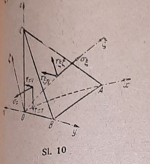
Figure 10
The condition of equilibrium of the forces acting on this tetrahedron in the direction of the ξ axis gives

If it is taken into account that
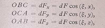
is obtained

and similarly from the conditions of equilibrium in the direction of the η axis:

These are the equations used for calculating stresses under coordinate transformation. Of particular importance is considering only those surface elements _dF for which the ξ-axis coincides with the z-axis. The formulas for this case can be obtained by simplifying the previous formulas or read directly from fig. 11:
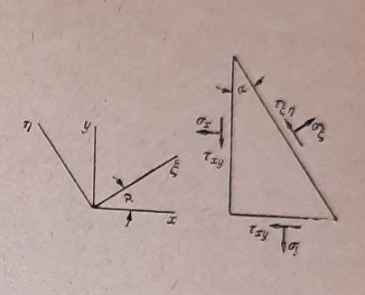
Figure 11

The normal stress takes extreme values for directions α = α0 , for which dσξ/dα = 0. By differentiation, from equation (16) we obtain

and therefore, when this expression is set equal to zero
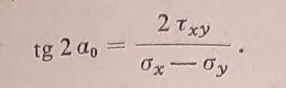
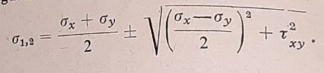
The stress τξη will also be the total shear stress in these planes, if τyz = τzx = 0. Then, by equation (17), two mutually perpendicular directions are determined for which: 1. the total shear stress is zero and, 2. the normal stress has extreme values (maximum and minimum). These directions are called the principal stress directions, and the corresponding stresses principal stresses. They are denoted by σ1 and σ2 and can be calculated directly from the formula
Mohr’s circle
The equations (16) can be represented graphically in an intuitive way. For this purpose they should be transformed into the form:
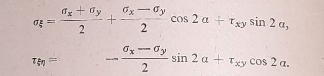
These equations represent, in the coordinate system σ, τ, the parametric form of the equation of a circle drawn in fig. 12, whose center coordinates are σ = 1/2 (σx + σy), τ = 0, and whose radius is
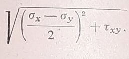
This circle is called the Mohr circle. If through point x a line parallel to the section x = const. is drawn, through which the stresses σx, τxy are transferred, it will intersect the circle at point p, called the pole of the Mohr circle. Any line pξ drawn through this pole intersects the circle at point ξ, which determines the stresses σξ, τξη transferred through a section parallel to pξ.
With regard to the sign of shear stresses when drawing the Mohr circle, care should be taken that they are plotted upward if they have the direction shown in Fig. 12c. Accordingly, of the two conjugate stresses τxy, τyx, one is always positive and the other negative.
The limit values of normal stresses σ1, σ2 correspond to points 1 and 2 on the circle, and the lines _p_1 and _p_2 give the directions of the principal stresses.
The representation of stresses lying in the x-y plane by means of the Mahr circle is not tied to any assumption about the stresses σz, τxz, τyz perpendicular to this plane.
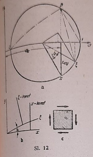
Image 12
This therefore also applies to the most general three-dimensional stress state, if only those cross-sectional planes are compared that all pass through the same straight line, which is here chosen as the z and ξ axis. Since according to the general transformation equations (15) the normal stress σ cannot become infinite for any cross-sectional plane, it must have a finite maximum σ1 for one plane and a minimum σ3 for another, both of which, of course, may also be negative. If a plane is drawn through the vectors σ1 and σ3 and the Mohr circle is drawn (fig. 13)
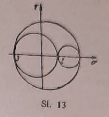
Figure 13
for stresses lying in this plane (i.e. all directions perpendicular to this plane), then σ1 and σ3 are the largest and smallest normal stresses that can occur and therefore must be mutually perpendicular. If the directions 1 and 3 are complemented by the direction 2, so that these three directions form a rectangular coordinate system, and if Mohr’s circles are drawn for the planes 1 ~2 and 2 ~ 3, then σ2 for one of these circles is the greatest, and for the other the smallest normal stress, and therefore in the sections perpendicular to the directions 1, 2 and 3 the shear stress is equal to zero. Three mutually perpendicular normal stresses σ1, σ2 and σ3, for which no shear stresses correspond, are called principal stresses.
Yield limit and failure limit under three-dimensional stress state
The state of stress is called one-, two- or three-dimensional, otherwise: linear, planar or spatial, depending on whether one, two or all three principal stresses are different from zero. In structural members most commonly used, i.e. in a tensioned, compressed or bent bar, the state of stress, at least at the most highly stressed points, is one-dimensional, as it is in tensile, compressive or bending tests, which in material testing are used almost exclusively for determining allowable stresses. By contrast, in plates loaded in their plane or perpendicular to it, as well as in shells, the state of stress is two-dimensional, and in certain cases three-dimensional stress states also occur, so it is necessary to draw conclusions about material behavior in the case of a spatial stress state on the basis of the yield and failure limits determined under a one-dimensional stress state.