Archival expert content: the text and formulas convey a historical theoretical presentation and are not a project, static calculation, load-bearing capacity check, assessment of an existing element, or instructions for construction or rehabilitation. Designations, assumptions and approximate patterns must be checked against the specific system, material, geometry, boundary conditions and applicable standards. Calculation of torsion, stability, fatigue, joints and stress due to prevented bending should be done by a licensed engineer, with independent control when required.
Today, Savo Kusić is focused on wooden windows, wooden-aluminum windows, custom windows, doors and requests for quotation. This article remains as a historical professional archive and does not represent a structural design service.
Saint-Venant torsion theory (free torsion)
Differential equation

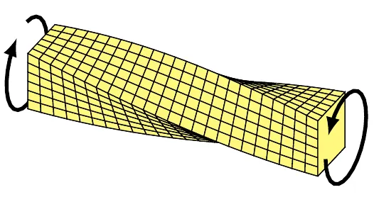
Sl. 1
Let a straight rod be fixed at one of its ends x=0 and let it be loaded at the other end with a torsion moment M (fig. 1). Then each of its sections rotates by a certain angle α(x) around a certain line parallel to the axis of the stick, which we will adopt for the x-axis. If all sections are equal to each other, each line parallel to the x-axis will pass into a coil, and the angle α will be proportional to the distance from the fixed end: α=ϑx, from which the component displacements in the plane of the section arise (fig. 2):
v = - r a sin__ψ = - ϑ x z,
w = r a cos__ψ = ϑ x y. (1a)
The quantity ϑ is called the torsion angle (dimension: length-1, rotation per unit of length). The torsion angle is proportional to the torsion moment M:
ϑ = M/GJT. (2)

Sl. 2
The proportionality factor GJT, torsional stiffness, is equal to the product of the shear modulus G and the factor JT, which represents the influence of the shape and size of the section.
This rotation of the section is not the only deformation of the rod. In addition, there is also bending of the cross-section, i.e. to the displacement u in the direction of the x-axis, which has the same magnitude for the corresponding points of all cross-sections and is therefore only a function of the coordinates in the plane of the section, and is otherwise proportional to the load M or the torsion angle ϑ:
u = u(y,z) = ϑ ∙ φ(y,z), dφ/dx=0. (1b)
If the expressions above are introduced into the corresponding displacement equations, it is obtained that the main normal stresses are equal to zero, so only two component stresses τxy and τxz remain:
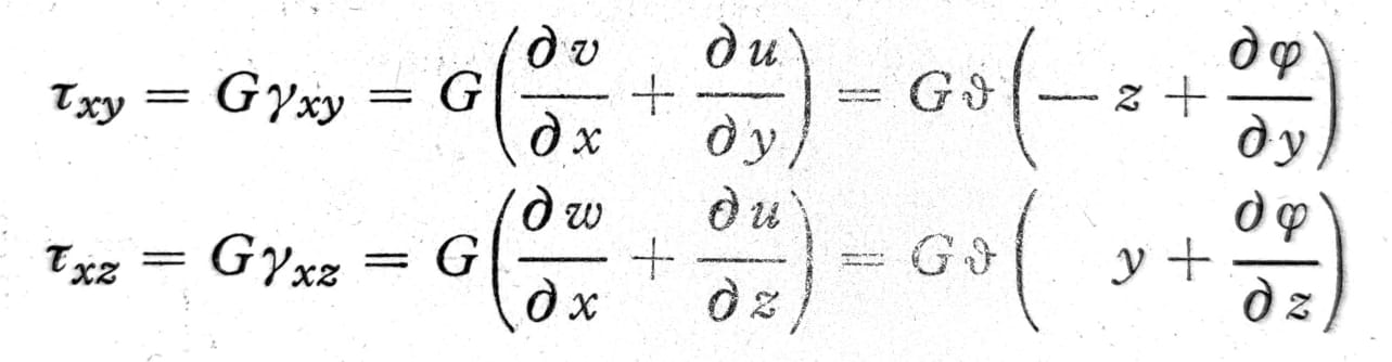
One. 3
The differential equation of the torsion problem is obtained based on the equations (3) by putting:
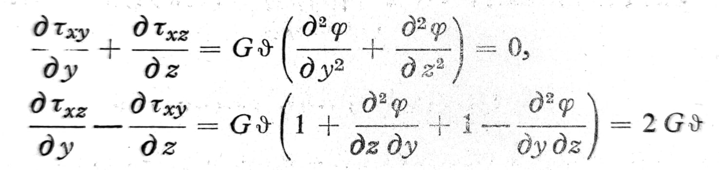
One. 4a and 4b
and solving these differential equations for the unknowns τxy and τxz by introducing the voltage function F(y,z) that:
τxy = - dF/dz, τxz = + dF/dy. (5)
With this, the equation (4a) is identically satisfied, and the required differential equation is obtained from the equation (4b)
d2F/dy2 + d2F/dz2 = 2G__ϑ (6)
The boundary condition required for the unique solution of this equation is obtained from the requirement that there are no shear stresses on the rod envelope, from which, due to the conjugate nature of the shear stresses, it follows that the stress in the section plane must not have a component perpendicular to it along the contour. From here, fig. 2:
dy/dz = _τxy/_τxz = - (dF/dz) / (dF/dy)
therefore
dF/dy dy + dF/dz dz = 0,
i.e. the total differential of the function F must be zero, that is, it must be F=const. along the contour.
If the section has only one contour, it can be simply put F=0 on it, because with the voltage function, of which we are actually only interested in derivatives, an arbitrary additive constant does not play a role. For sections that have more than one contour, this issue is more complex.
As can be seen from the equation (5), the resultant of the shear stresses τxy and τxz at an arbitrary intersection point is equal in magnitude to the gradient of the stress function F, but is perpendicular to it, i.e. has a tangent direction to the line F=const.
Solving the differential equation (6) yields the voltages τ as functions of y, z and ϑ. The task of the calculation is, of course, the determination of the torsion angle ϑ and the stress, especially the maximum stress as a function of the torsion moment, therefore, the determination of the stiffness of the section JT from the equation (2) and the resistive torsion moment WT = Mmaxτ. To obtain these, it is only necessary to express M as a function of F:
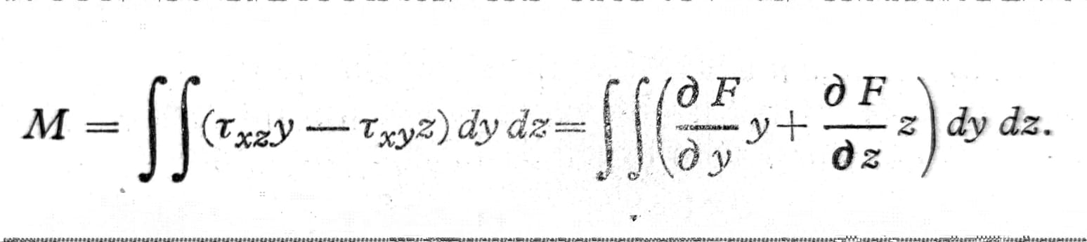
Both summations of this integral, which should be taken over the entire section, can be transformed by partial integration. If, for example, the first of them integrates first along the line z=const. from the point on the contour y=y1 to the point y=y2 (fig. 3) and taking into account that in both of these points F=0, we get
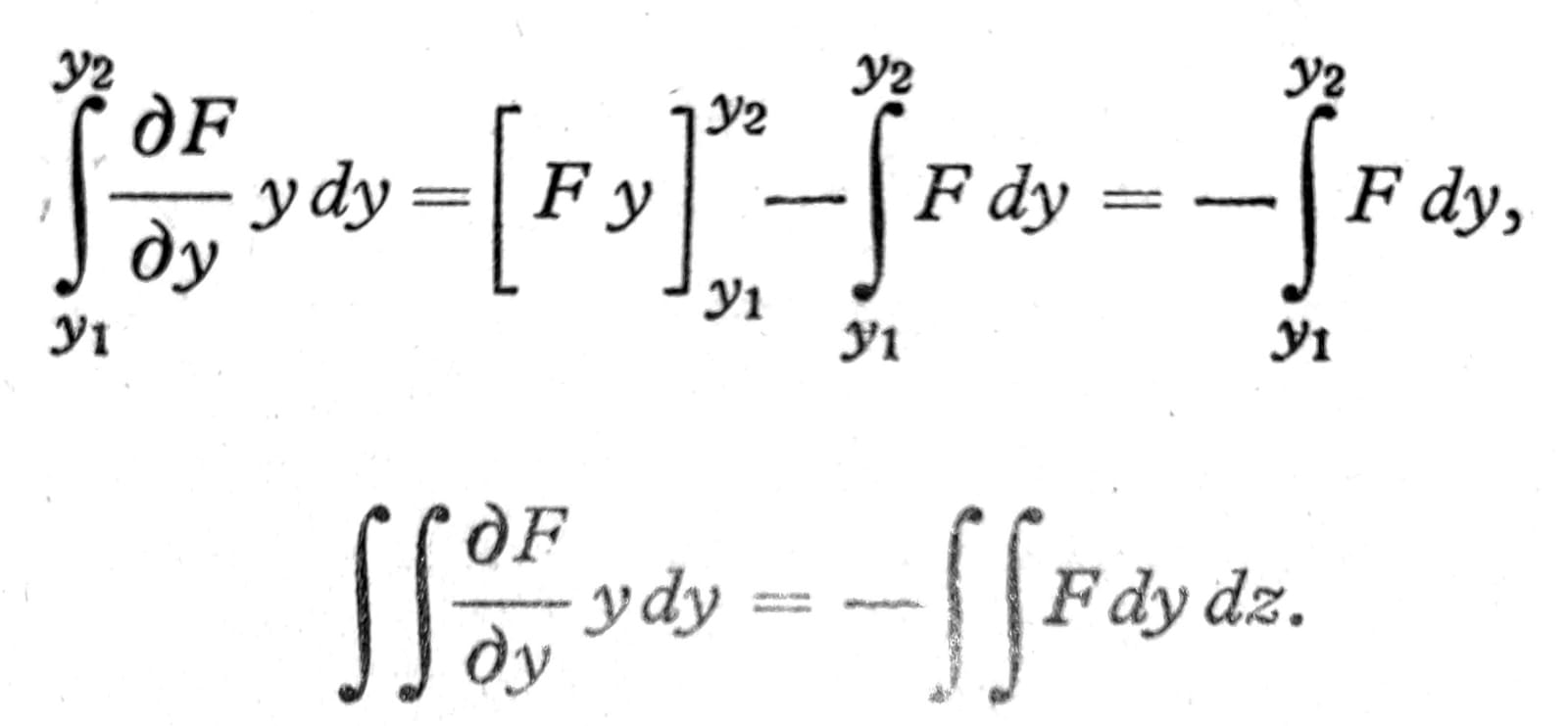
The same value is obtained from the second integral, so that
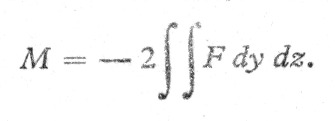
One. 7

Sl. 3
Other cases of full sections
The differential equation (6) is an inhomogeneous equation of potential theory. Therefore, for the solution of the torsion problem in the case of an arbitrary cross-section, the methods of the potential theory are available, which enable it to always be found. These methods, however, are generally too complex to be applied to individual cases that arise in practice. Therefore, the following table shows the results of such calculations for several sections.
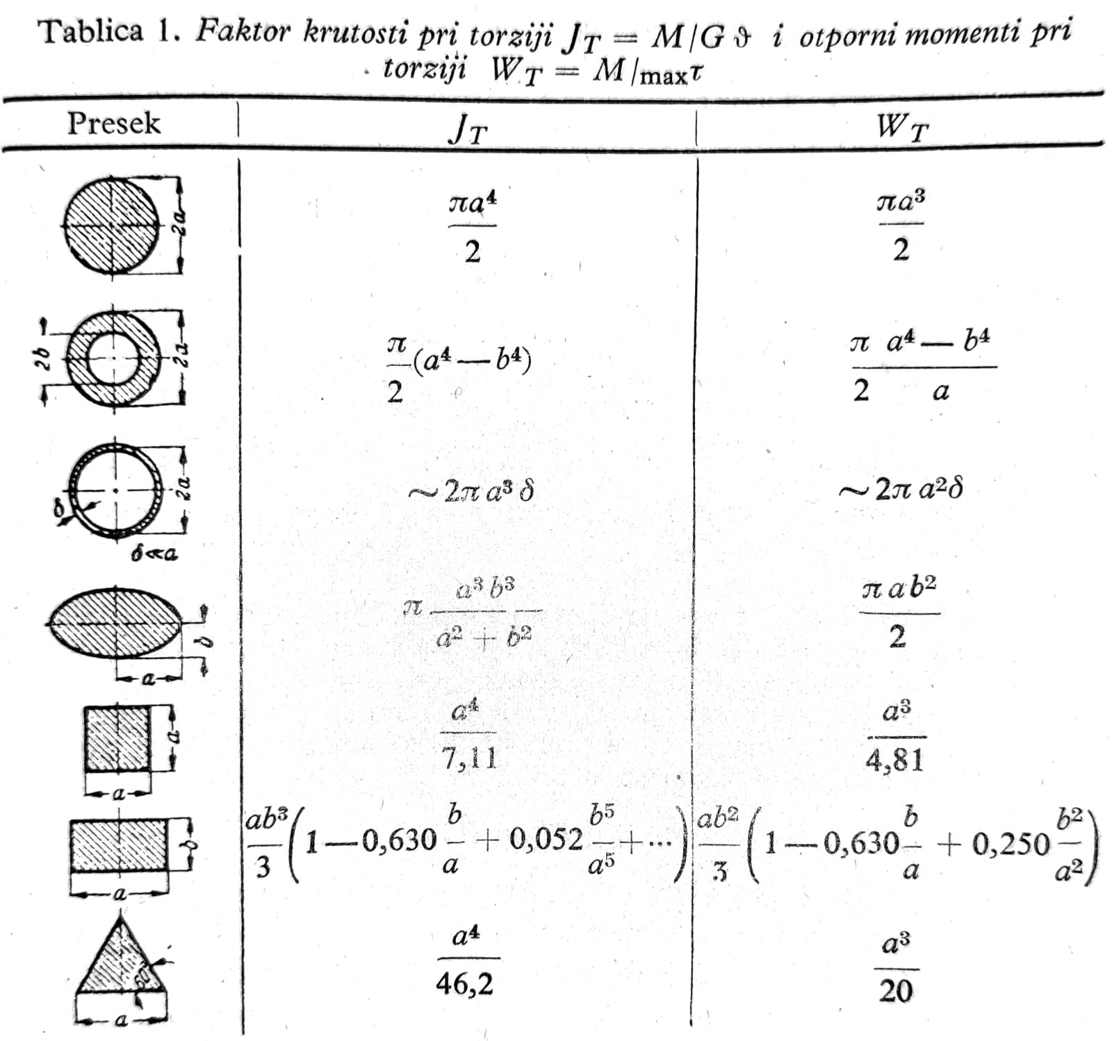
For sections close to circular, JT=F_4/40_Ip can be used, where F is the area, and Ip is the polar moment of inertia of the section.
Note on formulas and tables: expressions and values in scanned images are stored as a historical source. OCR text, index marks and scan are not reliable enough for calculation. Before use, each formula, unit, coefficient and area of validity should be checked in an authoritative professional source and applicable standard.
Analogy with the membrane
An analogy between the stress function F of the torsion problem and the deflection of a transversely loaded membrane provides a useful way to estimate torsional stresses and, at the same time, a procedure for determining them accurately. Let there be an opening in the flat wall of a vessel that is congruent with the cross-section of the bar subjected to torsion. When the membrane is stretched over this opening and a small excess pressure p is created in the vessel, the membrane bulges outward, so that its deflections ξ(y,z) satisfy the differential equation
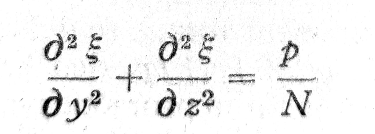
where N is the surface tension in the membrane caused by capillary forces (dimensions: force per unit length). This equation coincides with the equation (6), and the boundary condition ξ=0 is the same as for the voltage function. In this way, the voltage function F(y,z) can be obtained using this mirror with the membrane and thus solve the torsion problem. The stress τ corresponds to the slope of the membrane in relation to the y-z-plane, so the steepest place is the one where the rod exposed to torsion has the highest shear stress.
Sl. 4

Sl. 5
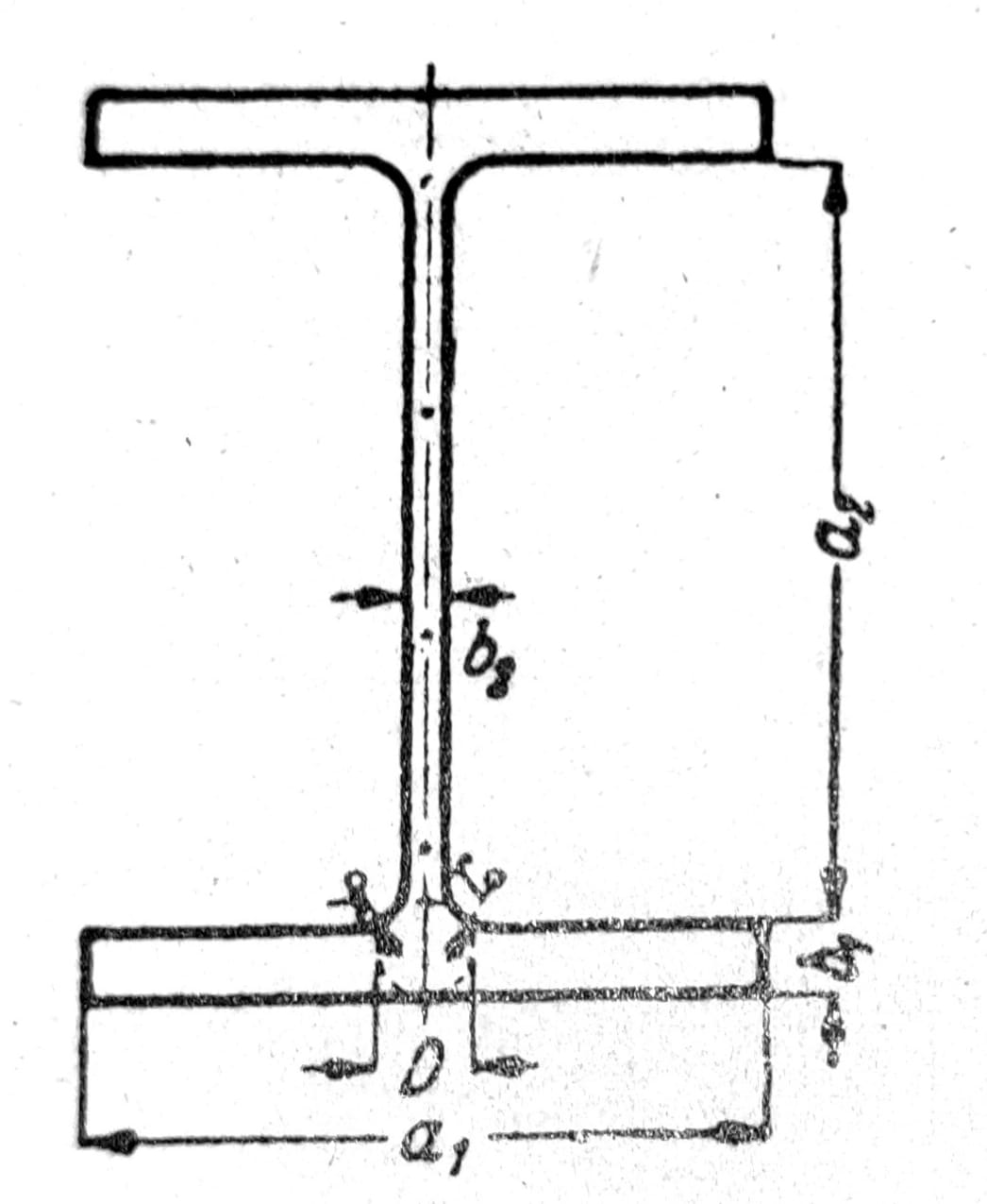
This membrane procedure is particularly suitable for obtaining approximate expressions for thin-walled sections. When, for example, the I-section is divided into three rectangles as shown in Figure 4 and the membrane analogy is applied separately to each of them, the sum of the volumes of the resulting protrusions will be only slightly smaller than the volume that actually corresponds to the stress function. Therefore, when the thicknesses b1 and b2 are small, approximately
JT = 2JT1 + JT2,
where JT1 and JT2 are stiffness factors of individual rectangles that can be calculated based on table 1. A better approximation is obtained when JT2 = a2 b32/3 is put for the rib, therefore, when the rib is considered as part of a very elongated rectangle. An even more accurate value is obtained according to Trayer and March\ from
JT = 2JT1 + 1/3 a2 b32 + 2 α D4,
where D is the diameter of the largest circle inscribed as shown in fig. 4, and α can be taken from fig. 5. For the T-section it is obtained similarly
JT = JT1 +JT2 + α D4,
where JT2 is half of the value calculated according to the table 1 for a=2 a2, b=b2. For L-sections (fig. 6) it is similar
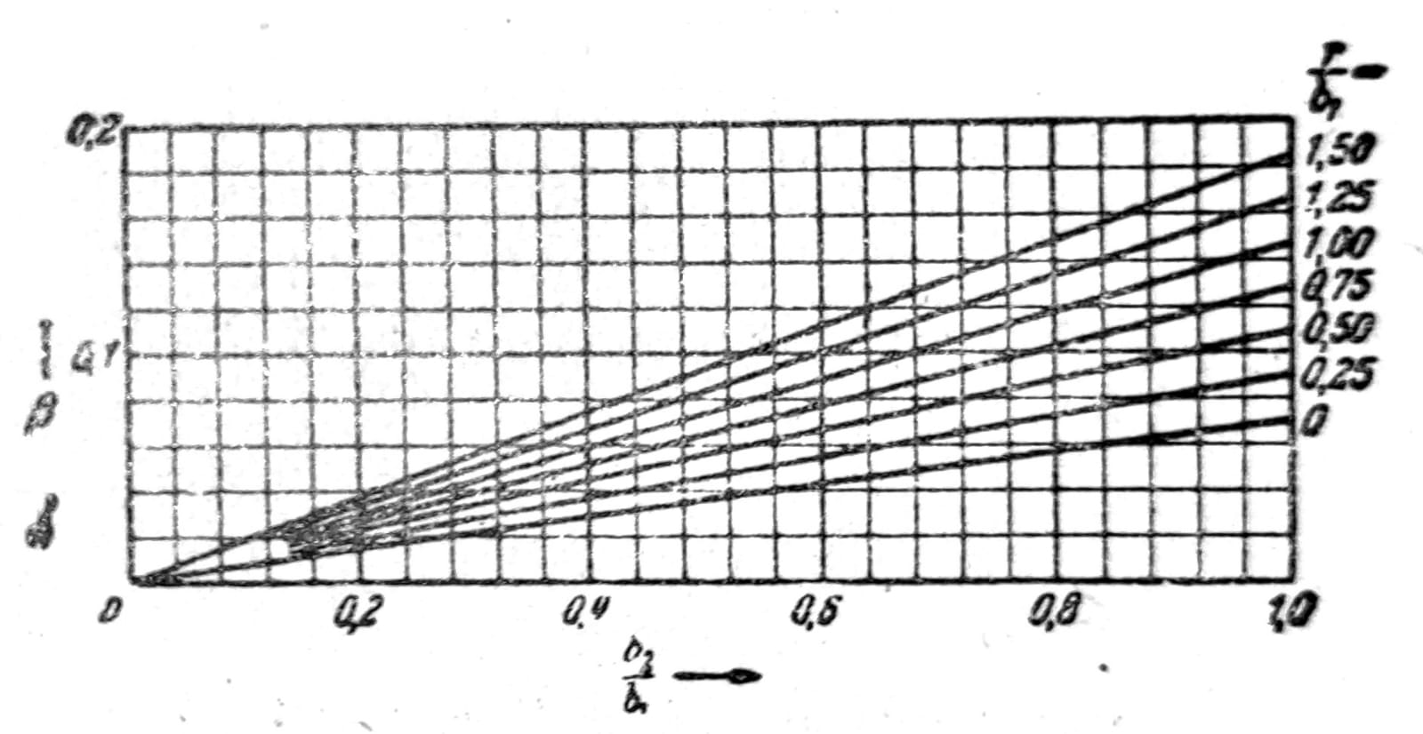
JT = JT1 + JT2 + β D4
where JT1 for the thicker arm is taken directly from table 1, while JT2 for the thinner arm is calculated as in the T-section, and β is taken from fig. 7.

Sl. 6
Sl. 7
When calculating the stress, the torsion moment is divided into constituent rectangles: the part that falls on the flanges M1=M JT2/JT; shear stress is then calculated at the middle of the longer side of each rectangle based on table 1. The largest of these stresses need not be the largest shear stress appearing in the section. Namely, if the angle of incidence is not rounded, τ=∞ is obtained at that place, so that for a very small radius of rounding, the highest shear stress can be expected here.
Engineering note: the mathematical singularity of the idealized acute angle is not a license to estimate the actual detail by this approximate pattern alone. The actual rounding geometry, tolerances, plasticity, welds, residual stresses, local stability and fatigue require appropriate modeling and expert verification.
For a one-sided angle whose side thickness is t according to Trefftz\ is on the rounding of the diameter r:
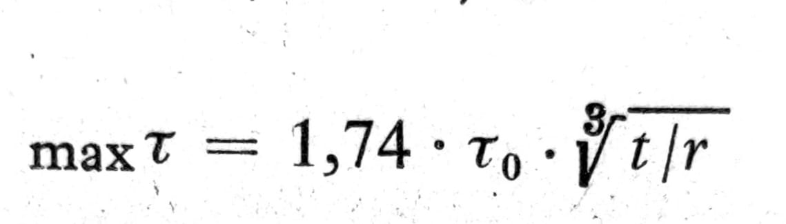
where τ0 is the highest voltage calculated for each individual leg based on the procedure described here. For larger rounding radii, τ=2__τ0 can be adopted.
Thin Walled Pipes (Bradt Patterns)
In thin-walled pipes, the bulging membrane has the shape shown in fig. 8, which consists of a plane above the hollow space inside the pipe and a sloping surface that surrounds it and lies above the effective section of the pipe wall; this inclined surface must be steeper if the pipe walls are thinner in the appropriate place. In this case, the shear stresses are distributed fairly evenly over the thickness of the walls and are inversely proportional to the thickness of the walls, i.e. shear force T = τt does not change along the circumference of the section.

Sl. 8
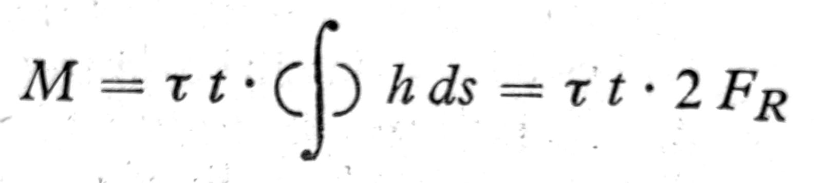
The surface element t_∙ds_ receives part of the torsion moment
dM = t_∙ds∙τ∙h,_
so the total moment is
One. 8
where the FR surface is covered by the middle line marked by lines and dots in fig. 8. It is obtained from here
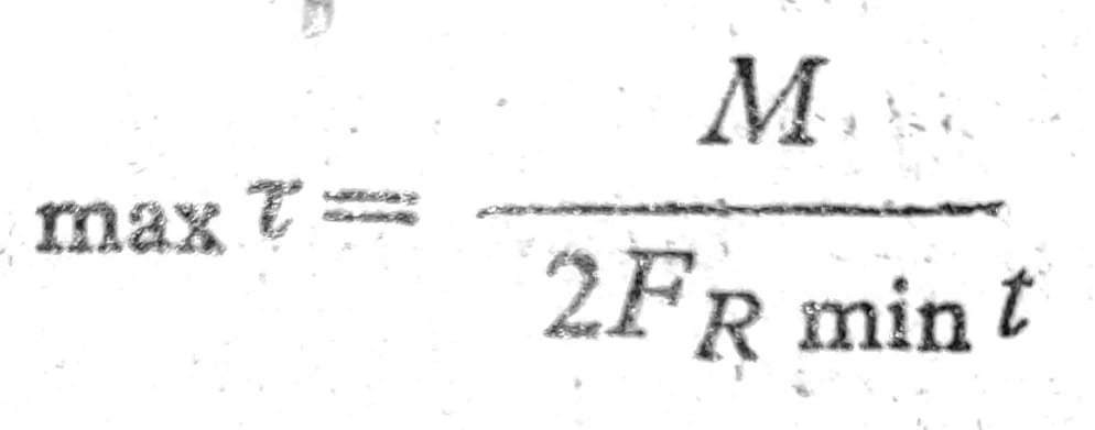
One. 9 - Bredt's first form
Torsional stiffness is obtained most simply when the deformation work is expressed on the one hand through torsion moment and torsion angle and on the other hand through shear stresses. In this way, it is obtained for a rod element of length l
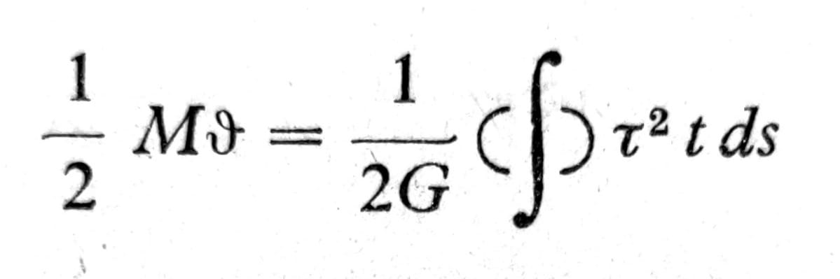
so, introducing the value for τ according to the equation (8),

that is, by comparison with the equation (2):
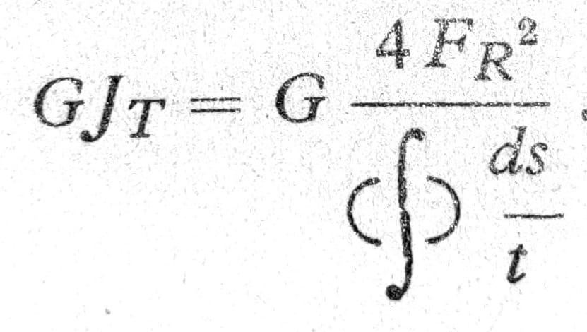
One. 10
If the thickness of the walls is the same all around, then it is simple (2. Bredt's formula):
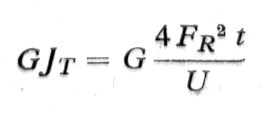
One. 11
Normal stresses in torsion due to section bending
Basic terms and differential equation
Component displacements u, equation (1b), determines the curvature of the sections from their planes. When the torsion moment is constant, this bending is the same in all sections and normal stresses σx do not appear.
In many cases, the curvature of the cross-section, which should arise on the basis of _St. Venant’s theory is not possible. If the torsional moment changes abruptly in one cross-section, bending of different magnitudes would occur on both sides of the cross-section, and the continuity of the deformation would be disturbed. One end of the rod can be so clamped that bending of the section is completely excluded at that point. In such cases, an amendment should be made _St. Venant’s theories. Additional stresses σx in the direction of the rod axis and additional shear force T (shearing stresses T/t) appear in the rod, which are highest in the section where the continuity of deformation is broken and which decrease exponentially with distance from this section. In the case of solid rods and tubes, this theory is complex, and the supplementary voltages decrease so quickly that their determination is not worthwhile in most cases. For thin-walled, open-profile rods, this correction is of great importance and can be calculated relatively easily.
Sl. 9
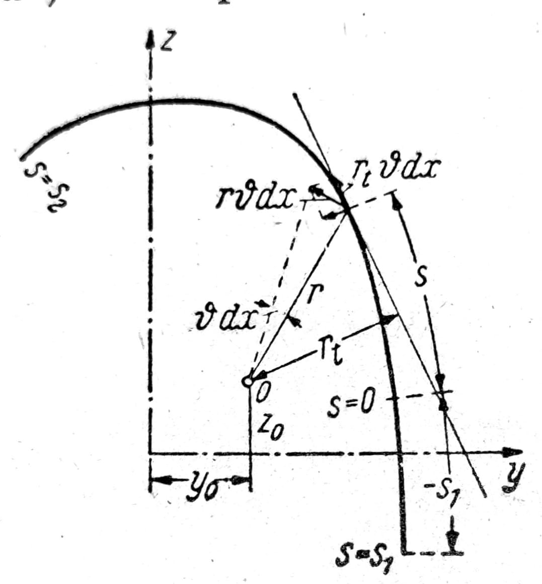
Sl. 9 shows the line along which the middle surface of the wall and the section plane intersect (the middle line of the section). O is the center of relative rotation of two adjacent sections. If their distance is dx, the torsion angle ϑ dx, then an arbitrary point of the middle line undergoes a displacement u ϑ dx. This displacement has a component rt ϑ dx in the direction tangent to the section, and is the slip of the element of the middle surface of the wall (considering that _u=_φϑ):
γ=__ϑ (rt + d__φ/ds).
Since the shear stress in the middle surface of the wall is zero, it must also be γ=0, and therefore
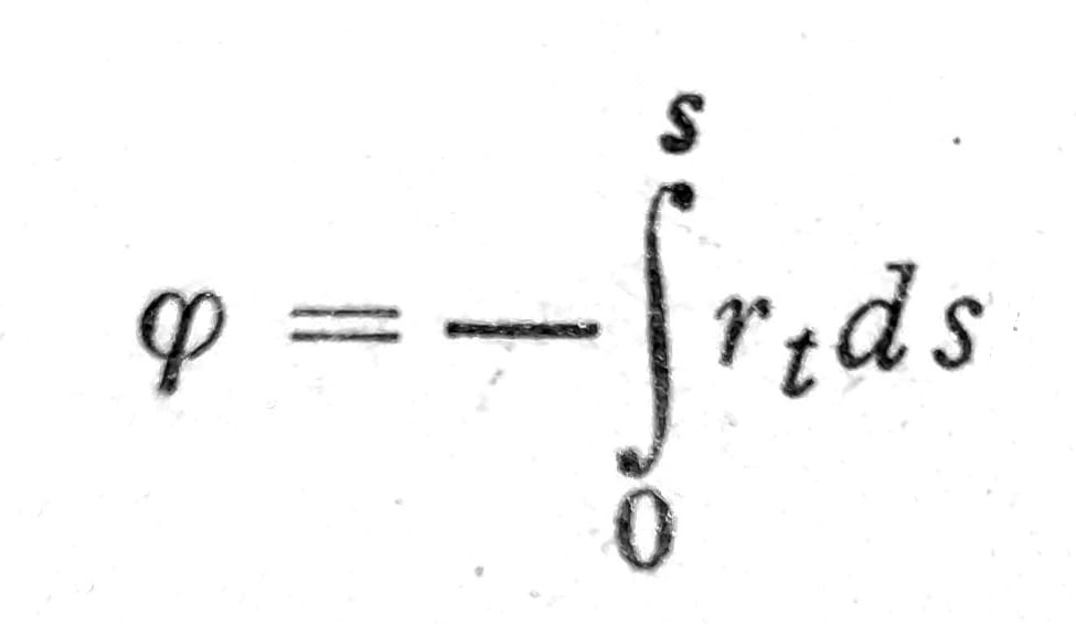
This form contains three arbitrary parameters: the start from which the arc length is calculated s and the coordinates of the center of relative rotation O, on which rt depends. The starting point from which the arc length s is calculated can be chosen so that the mean curvature value is zero:
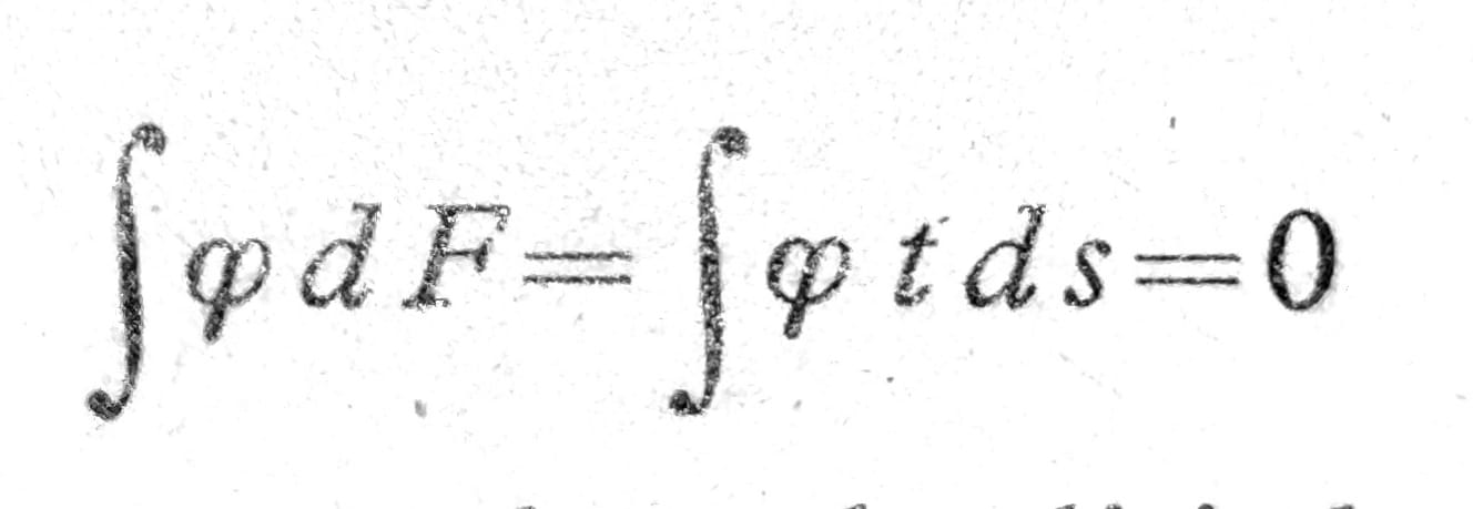
and the coordinates of the center O can be determined in such a way that the moments due to the bending of the section are zero:
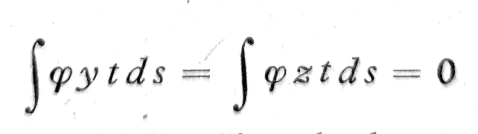
It can be shown that the center of rotation determined in this way coincides with the shear center described in the referenced discussion and defined in another way.
If the bending of the section described by these patterns is completely or partially prevented, normal stresses σx in the direction of the axis of the rod must appear. A closer study shows that these voltages can be taken to be proportional to the bending function φ: σx=k__φ, where φ depends only on s and k only on x. As per Hooke’s law:
σx = E_∂u/∂x = Eφ dϑ/dx_, (12)
must be k=E d__ϑ/dx. Normal stresses σx are called stresses due to section bending. Considering the equations above, they form an equilibrium system of forces in each section, a system of forces due to the bending of the section.
The total torsional moment consists of two parts: one of them M1=GJT__ϑ arises due to shear stresses during torsion which gives St. Venant's theory, and the second M2 occurs due to the bending of the section:
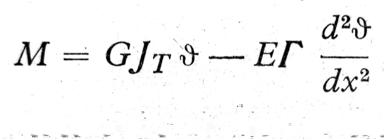
One. 13
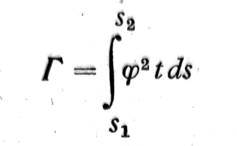
Since the moment M is given as a function of x, this expression represents a differential equation for the torsion angle ϑ. Once this equation is solved, M1 and M2 can be calculated, and thus all stresses and strains.
Solution and applications
When the torsion moment M is constant, the general solution of the equation (13) is:
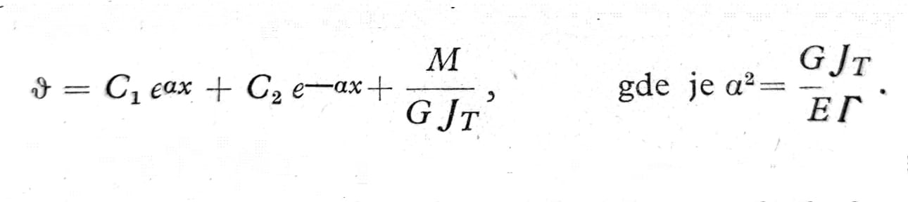
The integration constants C1, C2 must be determined from the two boundary conditions.
a) Rigidly clamped end x=0 (fig. 1)
At this end is u≡0, so based on equation (1b) ϑ=0. If the rod is very long (αl>>1), then C1=0 and C2= -M/GJT. In the case of short rods, the appearance of stress due to bending of the section is affected by the condition at the right end of the rod. If the bending of the section is not prevented at that place, there will be σx≡0 and dϑ/dx=0. It is obtained from here
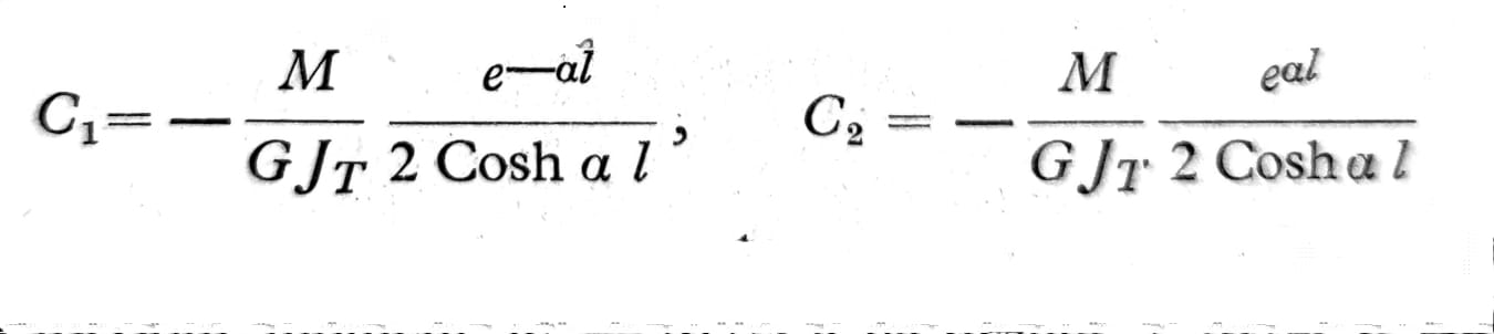
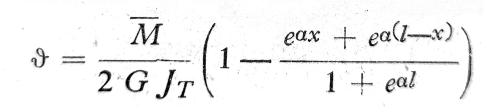
b) Symmetrical torsion load according to fig. 10
On the left half of the rod, the torsional moment is -M/2, and on the right +M/2. In the case of free torsion, the sections to the left and right of the middle of the rod would be twisted in the opposite direction, therefore the continuity of the deformation would not be preserved. Therefore, at the place x=0, the entire torsional moment must be transmitted through the stresses that occur due to the bending of the section, and therefore in this section M1=0 and therefore ϑ=0. At this point, a system of forces acts to ensure that the section remains straight, even though sections that lie farther from the center of the rod curve. If, in addition, it is required that the ends of the rod have stresses σx≡0, one more boundary condition is obtained for each half of the rod, so for the right half

Sl. 10
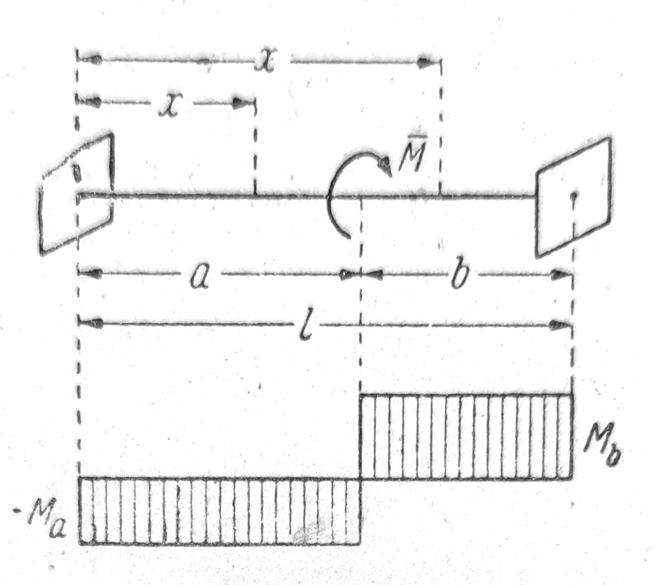
c) External moment M at an arbitrary place (fig. 11)
In this case, the solution ϑ for both parts of the rod must be written separately, so a total of four constants C1, C2, C3, C4 appear. In addition, the torsion moments Ma, Mb are also unknown. Six equations are available: a continuity condition for ϑ (expressed by u) and for dϑ/dx (expressed by σx) at the point of action of the load, one condition at each end of the rod (e.g. rigid pinching ϑ=0, or undisturbed bending, dϑ/dx=0), the condition of balance by moments -Ma+Mb=M and finally the condition that the end sections do not rotate towards each other: ∫ ϑdx = 0.
Sl. 11
Final note: the choice of torsion model depends on the open or closed section, slenderness, method of support, place of moment input and the possibility of free bending. For a real element, the load-bearing and serviceability limit states, local details, joints, fatigue and stability must be checked, not just one isolated formula from the article.