Today, Savo Kusić is focused on wooden windows, wood-aluminum windows, custom windows, doors and requests for quotation. This text remains as an archive of structural theory and is not an offer of static design, stability calculations or structural rehabilitation.
Differential equation of buckling in bending
It is assumed that all idealizations are satisfied, in particular
- that the member is perfectly straight
- that the load P acts along the member axis
- that the stresses remain below the proportional limit
- that the deformations are small enough for the usual calculation simplifications.
If the member bends under force P and possibly also under the transverse load q, the familiar equilibrium conditions between the external loads and the internal forces in the section must be satisfied. The established relationships between deformation and internal forces in the section must also hold.

Fig. 1 - Equilibrium
Fig. 1 shows a curved member element of length ds. The slope of tangent v’ is small, so, up to second-order terms, the element length may be taken as equal to its projection ds=dz. The following analysis also excludes cases in which P continuously changes along the member axis, so the axial force is N≈P=const. A number of terms in the three equilibrium conditions for the element may then be neglected. Using the notation and signs from fig. 10, the first approximation gives
N=P, M’=Q, Q’=-q+Pv’’.
The shear force can be eliminated, giving M’’=Pv’’-q. The Bernoulli relation M=-EI/R provides the remaining equation. As usual in beam-bending theory, the curvature of the member axis is simplified as follows
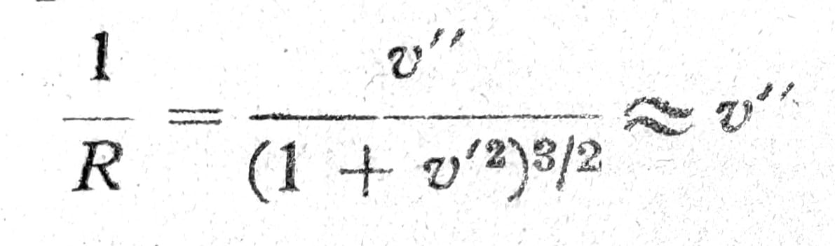
The bending moment can therefore be eliminated; with M=-EI*v’’, the differential equation for the bent member becomes
(EI*v’’)’’ + Pv’’ = q. (1)
In the special case of constant bending stiffness EI=const. the equation (1) is simplified so it is
EIv’’’’ + Pv’’ = q. (1a)
Equations (1) and (1a) are linear in v under the stated simplifications.
Practically, the simplest case of constant bending stiffness EI=const., which serves as the basis for the examples below, is particularly important.
Euler’s case
In addition to the stated idealizations, the assumptions for the classical buckling case are p=0, hence N=const.=P, and constant stiffness with frictionless hinges lying exactly on the member axis. The ordinary differential equation (1a) is fourth order, linear and homogeneous because q=0. Its general solution is:
v(z) = A_∙_sin__αz + B∙cosαz + C∙z + D, (2)
where A, B, C, D are the four constants of integration. The parameter is of finite size due to the assumption EI≠0. Furthermore, α≠0 holds for P>0.

Fig. 2
Since the linear differential equation (1a) is homogeneous, n_∙_v(z) is also a solution, where n is an arbitrary constant. The mathematical classification of the differential equation (1a) already shows that the magnitude of deflection v cannot be determined. To determine the integration constants A, B, C, D in the Euler\ case (fig. 2), the following boundary conditions are available: at both pin-ended supports the deflection and bending moment are zero, namely
v=0 and M=0 for z=0
v=0 and M=0 for z=s.
Since M=-EI_∙__v’’_, the condition M=0 gives v’’=0, so the four boundary conditions are:
v=0 and v’’=0 for z=0
v=0 and v’’=0 for z=s.
The solution (2) thus results in four linear equations:
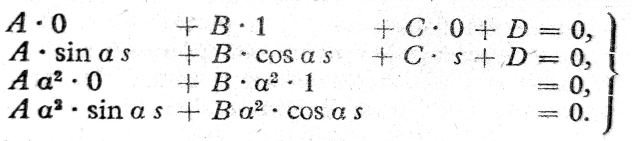
Eq. 3
These four homogeneous equations have the so-called trivial solution A=B=C=D=0, corresponding to v(z)=0. The straight member v_(z_)=0 is the usual equilibrium position for arbitrary, and especially smaller, values of load P. The conditions of interest here are those under which the member deflects, so that v(z)≠0. The equations (3) have a non-trivial solution with A, B, C, D ≠ 0 only when the determinant of the coefficient matrix is zero.
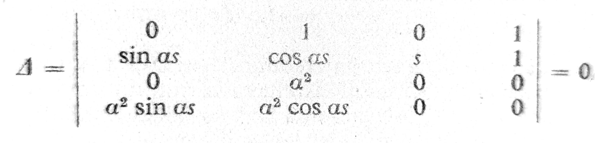
Eq. 3a
From the buckling condition Δ = α4∙s∙sinαs = 0 the critical values of PK load can be calculated. This equation is satisfied only if sin αs = 0, i.e. for αKms = mπ with m=1,2,3,… The corresponding values of Euler's buckling force are PKm=EI_∙_α2Km = EI(mπ/s)2. For each value of m, a certain buckling force is obtained. In most cases, only the smallest of these forces is of interest, and that
PK1=EI(π/s)2.
In what follows, the index m, or 1, referring to the lowest critical load is usually omitted. The corresponding elastic curve is of interest. From equation (2), the constants B=C=D=0 are obtained, while the condition A∙sin__αs=0 remains. For the case m=1 above, the elastic buckling curve is therefore v(z) = A_∙sinπz/s_, where v(z) is the eigenfunction corresponding to αK or PK. The magnitude of A remains undetermined.
Consider the entire load range again. For arbitrary values of P, particularly for forces P_<_PK1, v(z)=0 and the member remains straight.
By “gradually increasing” loading P is meant in the classic theory of stability a consecutive series of quantities P, where the stability of the observed load case will be tested over and over again for each individual load level P. During the stability test, the value of P certainly remains unchanged. If one state P is found to be stable, then the load is increased by something, and therefore the stability test is repeated. This accurate determination is necessary so that there is no confusion with the type of load, which is the basis for the Shanley\ effect, in which there is an increase in the load while small disturbances are acting at the same time. When examining the stability according to Shanley, in the area of plastic buckling, a smaller bifurcation force occurs than with the classical method of consideration.
The following considerations assume the first way of increasing the load: At a gradual increase of the load P in this sense, for PK1=EI_∙(π/s)_2 you first arrive at one bifurcation point of the elastic equilibrium, with a simple sine line as the elastic buckling line
v1(z)=f_∙_sin__π__z/s.
f=A denotes the undetermined amplitude of the elastic curve. For loads _P*__>_PK1, the linearized theory gives Δ≠0, so equilibrium is not possible there. Only at higher buckling loads PK2 etc. does Δ=0 occur again and hence also v(z)≠0. The reason this theoretical conclusion does not match actual behavior lies in the linearization of the differential equation.
Buckling of built-up compression members composed of two parts
The discussion is limited to compression members composed of two parts; similar relationships apply to compression members made of three or more parts.
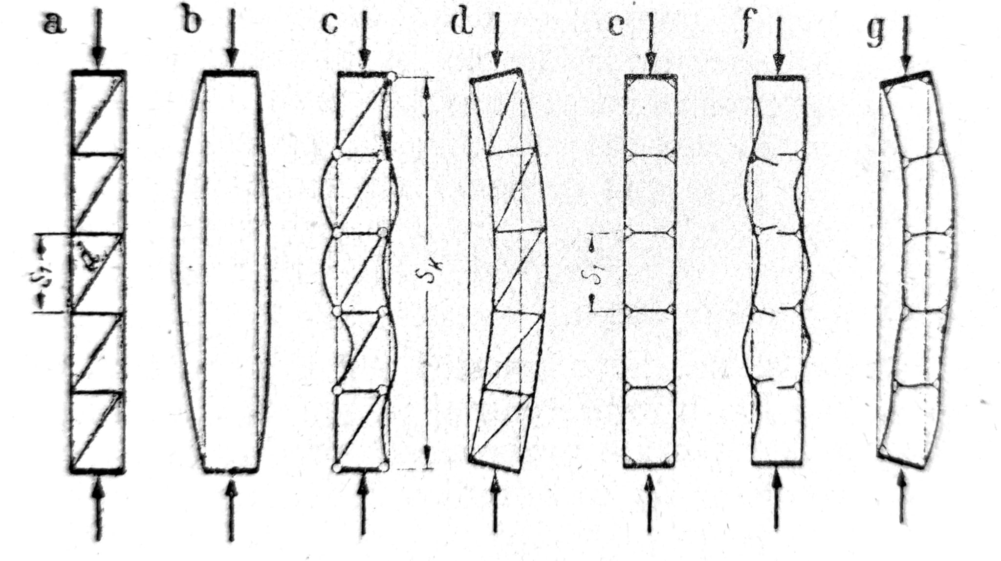
Fig. 3
According to the type of transverse connection, latticed members (fig. 3a) and battened members (fig. 3e) are distinguished. Without transverse connections, each component would buckle independently (Fig. 3b). If the web system is relatively flexible, an individual chord may buckle without the member as a whole deflecting. For the latticed member in fig. 3c, compare the pin-jointed system on the left with continuous chords on the right; for the battened member in fig. 3f, compare flexible connecting plates on the left with rigid connecting plates on the right. The slenderness λ__1_=s1/i1_ therefore has a major influence. For an individual component, I1=F1_∙_i12; s1 is the panel spacing (fig. 3), and i1 refers to axis 1-1 (see fig. 4).
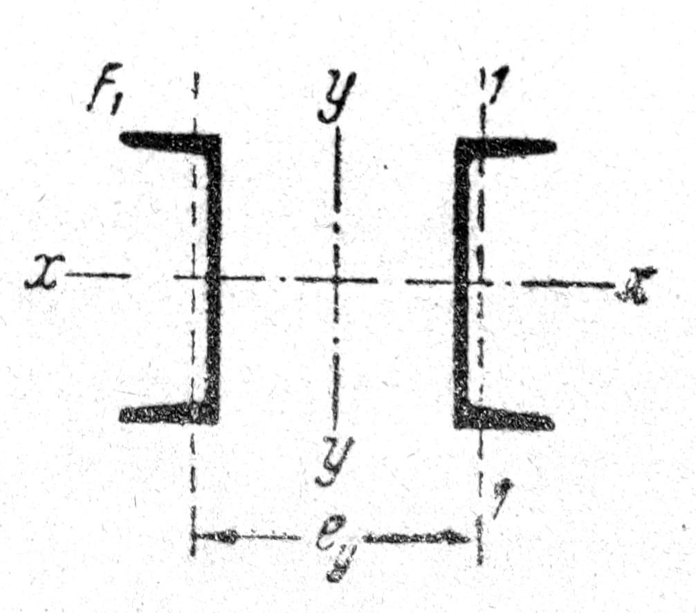
Fig. 4
The buckling load of built-up members corresponding to the elastic buckling curves in fig. 3d or 3g has been the subject of extensive theoretical investigation. If the member had a solid cross-section (for example, with a web), or if the transverse connections were so closely spaced that the two-part member did not differ in its behavior from a solid member, then σ__K_=_π__2__E/λ__y__2. Here λ__y=sK/iy (fig. 4). This buckling stress is not fully reached in practice because the transverse connections are neither infinitely numerous nor rigid. A satisfactory approximation for most cases follows the proposal of F. Engesser, according to which the buckling stress of a compression member composed of two parts is
σ__K_=_π__2__E/λ__yi__2.
λyi is the so-called ideal slenderness.
The transverse connections must be sufficiently numerous and strong to make both parts of the member act together. Neglecting secondary stresses, the transverse connections remain unloaded while the member is straight. Once buckling begins, they must carry forces and transmit shear forces that increase with deflection. If the elastic curve is
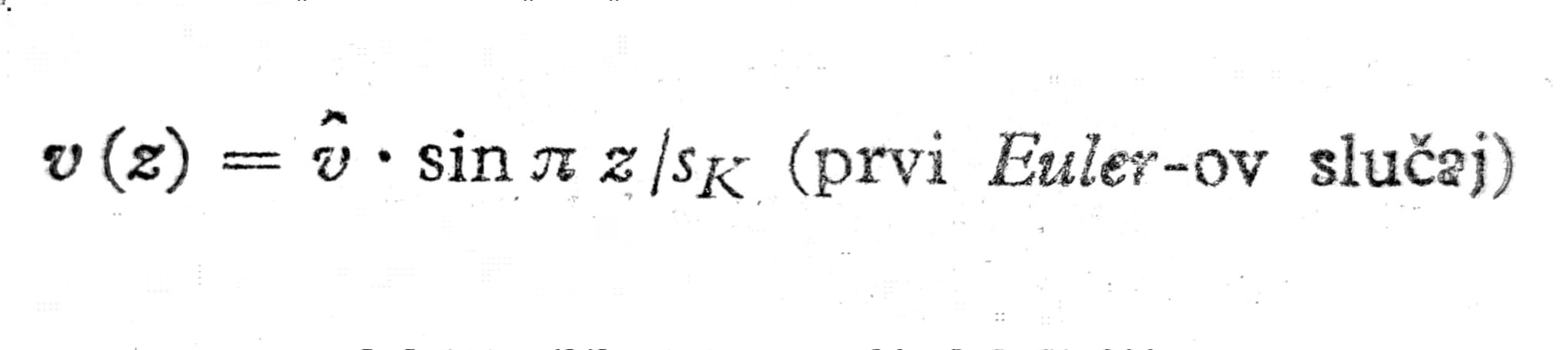
the shear force for I=const. is
Q = M’ = - EI∙v’’’.
From fig. 5, Q(z)=PK∙v’(z) can be read directly. Its largest value at the end of the member is
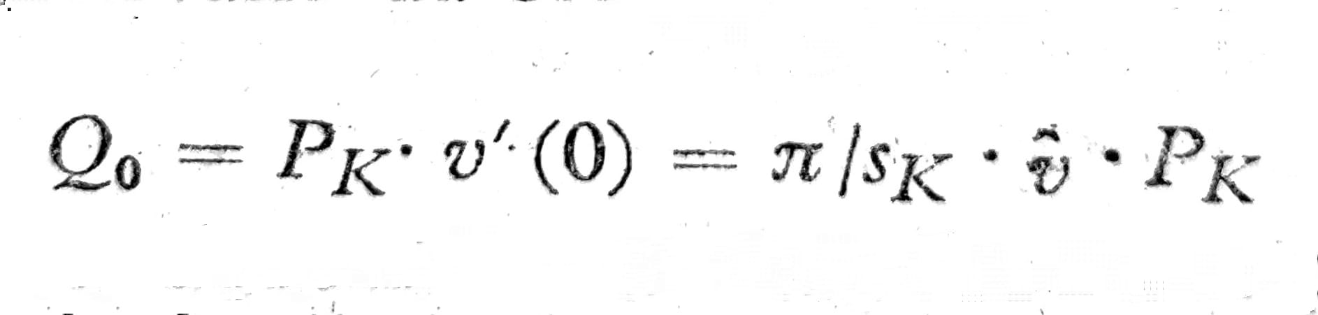
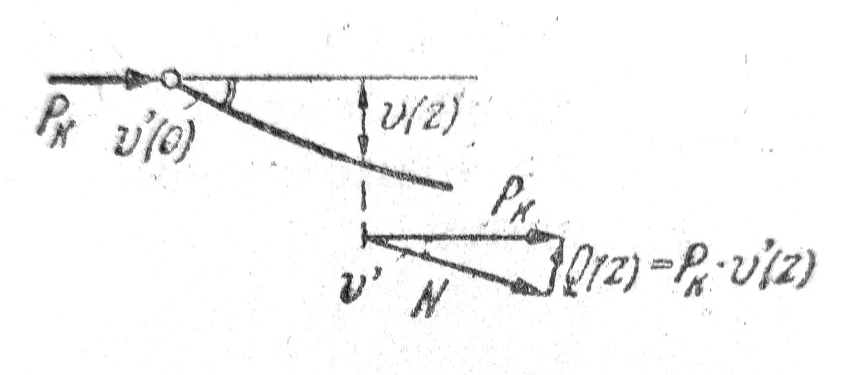
Fig. 5
The transverse connections must be capable of carrying this shear force. Since the corresponding load is the buckling load PK, it is sufficient for the transverse connections to reach their resistance at the same time as the member as a whole. There is no benefit in designing them much stronger than required for Q0; connections that are too weak, however, would cause premature member failure.
The equation above cannot initially be used because the magnitude of lateral deflection is unknown. Under PK the member is in neutral equilibrium and, at least in the first approximation, may assume an arbitrary deflection. Following F. Krohn, it is therefore useful to determine the deflection maxv at which the buckled member loses its load-bearing capacity through flexural failure. This will occur when the yield limit is reached on the concave side of the bend (fig. 6). Further deflection then increases while the corresponding bending moments cannot be sustained.
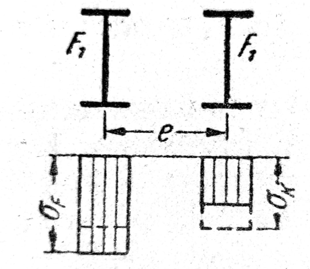
Fig. 6
For an ideally plastic material, the total stress on the concave side of the bend is, according to fig. 6,
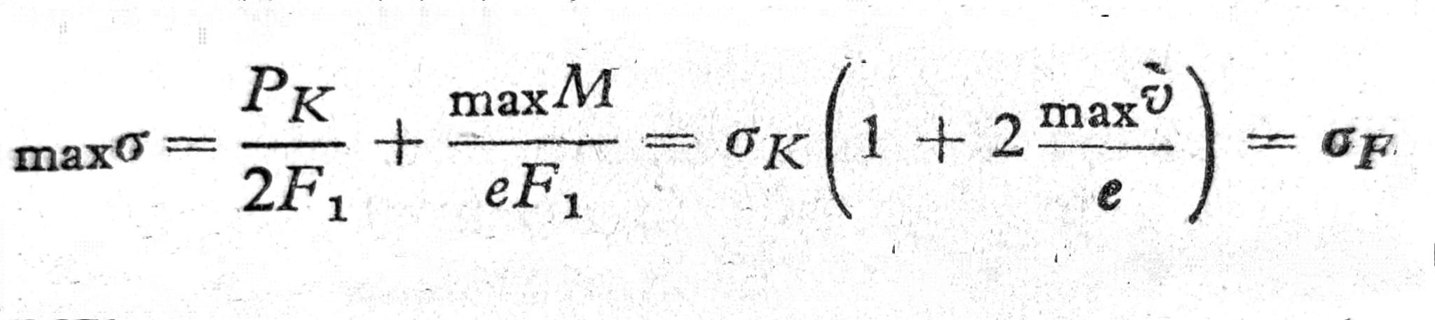
This gives the greatest deflection that can still be sustained
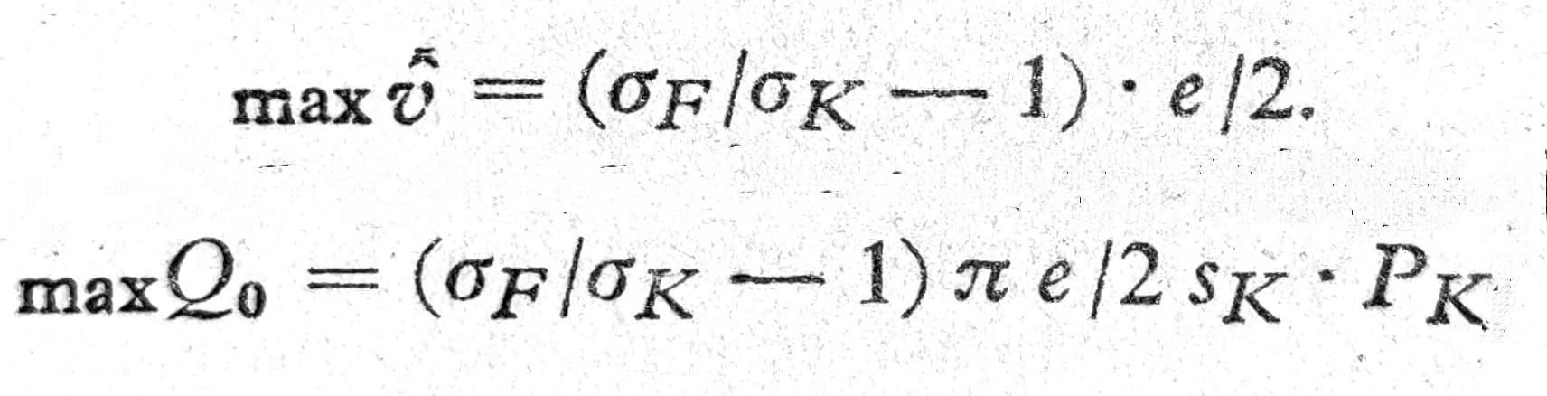
maxQ0 is the corresponding shear force at the end of the member.
If used for σK Tetmajer's form and put σF=3,1 t/cm2 and sK=e/2 ∙ λy which corresponds iy≈e/2, then Krohn's approximate value maxQ0=F/28 (Q in t, F in cm2) is obtained.
For arbitrary buckling-stress curves, one obtains
maxQ0=μK∙SK.
The coefficient μK varies with member slenderness and also depends on the material. Dividing the equation above by the safety factor against buckling gives
dozv__Q=μ∙dozvS.
Buckling of member systems
For member systems, it is customary to determine, for comparison, the buckling length sK=β∙h of a pin-ended member whose buckling load PK=π2EI/s2K is equal to that of the system. The equivalent “buckling length” is given for the examples below.
a) Rod clamped at both ends (EI=const.)
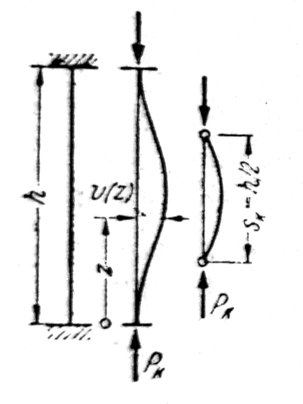
Fig. 7
For the case of fig. 7 of buckling is PK=4π2EI/h2=4,0∙PE, the comparative “buckling length” sK=h/2 and the elastic line of buckling v(z)=D(1-cos2πz/h).
b) Rod free at one end (fig. 8)

Fig. 8
It is assumed that the direction of P does not change as the member deflects. Then (EI=const.)
PK=π2EI/4h2=PE/4, sK=2h
v(z)=D(1-cosπz/2h).
The boundary conditions at the free end z=h are
M=0 or v’’=0
Q=M’-Pv’=0 or v’‘’+a2∙v’=0.
c) Rod clamped at one end (fig. 9)
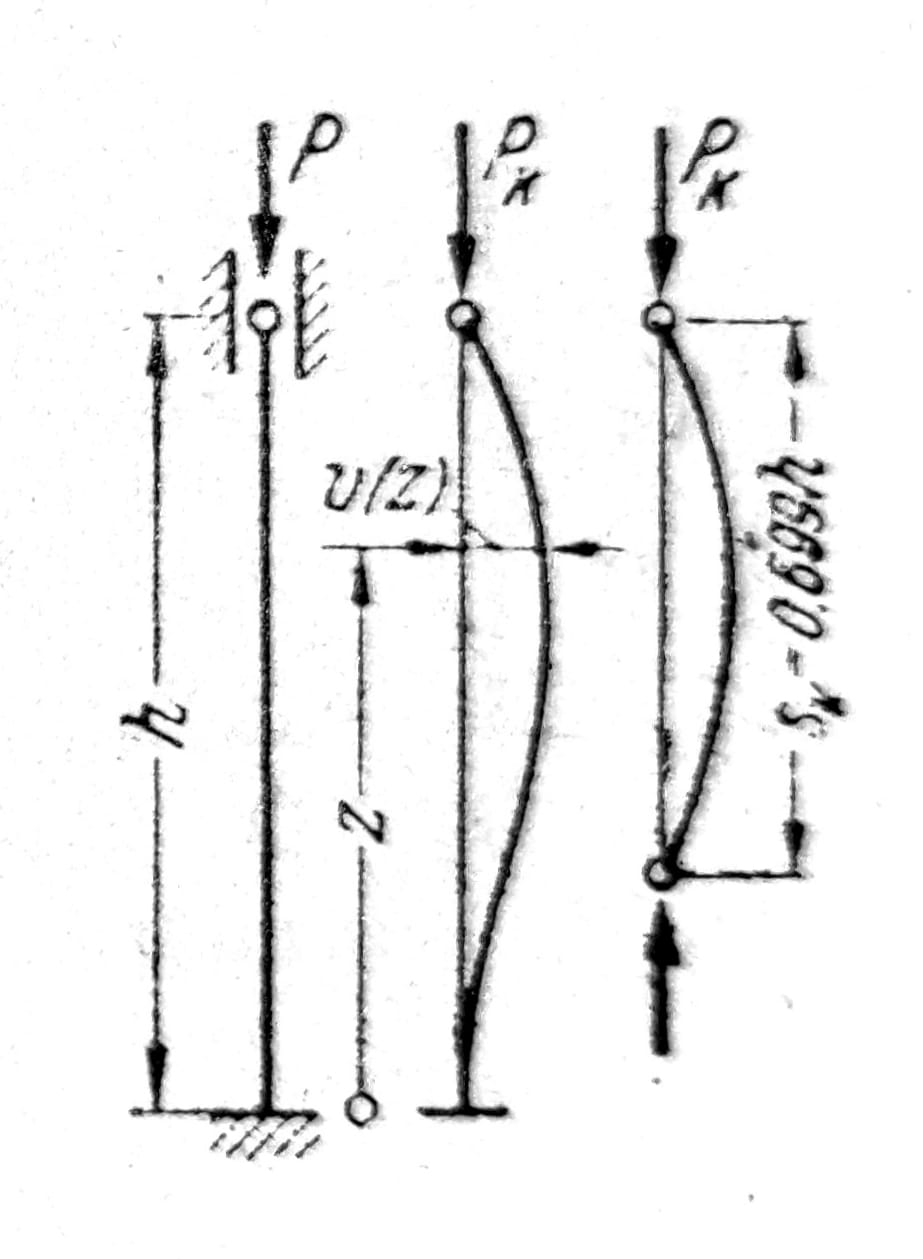
Fig. 9
With the boundary conditions
v=0 and v’=0 for z=0
v=0 and v’’=0 for z=h
is obtained for EI=const. buckling condition
sin_αh - αh∙cos_αh=0_,_
or equivalent
tgαh=αh. (4)
The roots of this transcendental equation are found in tables K. Hayashi's. The lowest buckling force is according to the tables PK1=4,49342/h2 ∙ EI = 2,046 π2EI/h2.
The comparative buckling length is sK = h / √2,046 = 0,699h.
d) Member clamped at one end with an imposed displacement (fig. 10)

Fig. 10
Consider a prescribed tip displacement of constant magnitude. The boundary conditions are
v=0 and v’=0 for z=0,
v=v1 and v’’=0 for z=h.
It is an equilibrium problem with an elastic line
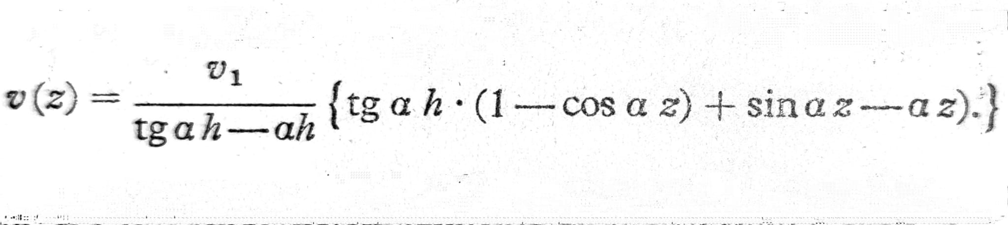
The denominator of the term before the {} brackets becomes zero and deflections grow without bound as P→PK (see buckling condition Eq. (4)). A characteristic feature is that deflections at the middle and lower part of the member initially decrease as load P rises and change sign only at higher loads. Fig. 10 shows deflection at half height.
e) Continuous member over two spans
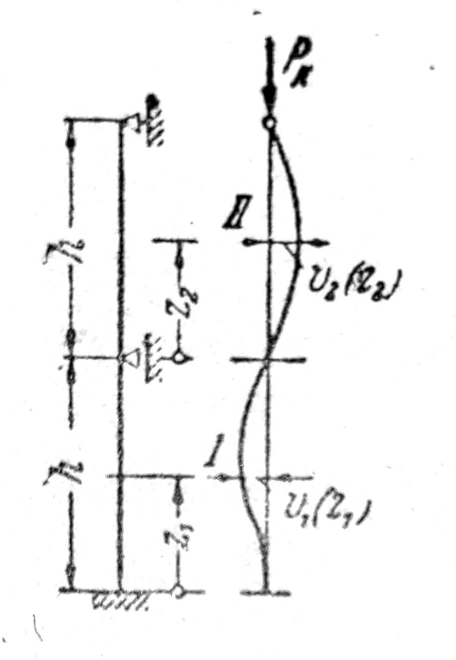
Fig. 11
For both solution regions (fig. 11), use the assumed form
I_. v(z1) = A1∙sinαz1 + B1∙cosαz1 + C1∙z1 + D1,_
II. v(z2) = A2∙sinαz2 + B2∙cosαz2 + C2∙z2 + D2.
For simplicity, let (EI)1=(EI)2=EI. The eight constants A1, …, A2, … are found from the boundary conditions
v=0 and v’=0 for z1=0,
v=0 and v’’=0 for z2=h,
as well as transitional conditions between areas I and II
v=0 for z1=h and for z2=0,
v’’(z1=h)=v’(z2=0),
v’’(z1=h)=v’’(z2=0).
The conditional equations are given in the table below

By setting the determinant of the coefficient equal to zero, the buckling condition is obtained
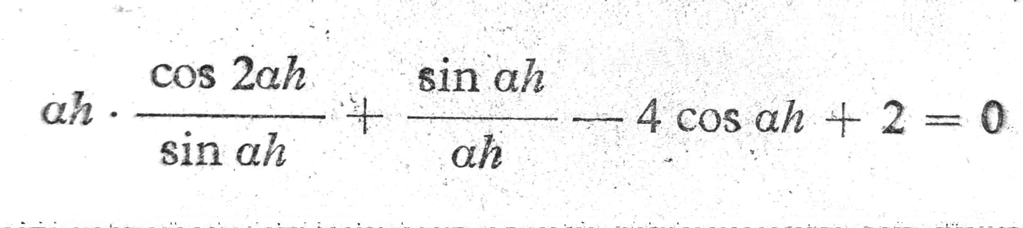
The buckling length is sK=0,878_h_, whereas for fig. 35 it was β=0,699. The buckling load decreased from 2,046 to 1,297 because a second pin-ended span was added. If the second span were clamped at its upper end, the buckling load would rise again to approximately 2,04 PE.
This historical presentation of formulas is neither a design nor proof of structural stability. The classical assumptions of a perfectly straight member, concentric load and elastic behavior do not necessarily cover initial imperfections, residual stresses, eccentricity, connection stiffness, material nonlinearity, lateral stability or, where relevant, fire, seismic action and erection stages. An authorized structural engineer must design the actual structure in accordance with current codes and standards.