Important professional note: This article is an archival educational review and is not a geotechnical study, valid laboratory standard, foundation calculation or execution instruction. The original terms, procedures, units of measurement, values, classifications and references to “our regulations” were transferred without checking compliance with applicable standards and regulations. Soil testing, choice of method, interpretation of results and design decisions must be carried out by authorized geotechnical experts and the appropriate laboratory for a specific facility and location.
The subject of soil compressibility is not part of the new public offer of Savo Kusić. The current production focus consists of wooden windows, wooden-aluminum windows and custom-made doors. For a specific window or door project, you can send a request for quote.
The basis of the oedometer test
The compressibility of the soil is determined by a compression test with prevented lateral expansion, which is also called an oedometer test or a consolidation test.
The test is performed with undisturbed samples, and in some cases with disturbed ones. In the first case, the test sample is taken by pressing metal rings into a larger, undisturbed sample, which is then fed into the apparatus together with the ring after cutting off the excess sample and leveling its surfaces with the edges of the cylinder. In the second case, the ring is filled with the sample in a state of consistency at the yield point and in that state it is introduced into the oedometer.
The test is carried out using the apparatus that was first constructed by Terzaghi and called the Oedometer. Today, there are several different constructions of this apparatus, but they are all based on the same principle, testing the compression of a soil sample under load with prevented lateral expansion.
Oedometer: description of the device

Sl. 1. Oedometer
The oedometer consists of a metal cylinder in which the sample is located between two filter stones (fig. 1). The sample is introduced into the apparatus in a metal ring with a diameter of 7-10 cm and a height of 1-4 cm. The load P is transferred to the sample via the upper filter stone. Below the lower filter stone, there are channels in the bottom of the cylinder for draining water from the sample into the capillary tube, as well as for water supply. Since the compression of the sample is done at the expense of the pores, because solid soil particles and water in the pores are practically incompressible, it is necessary during the test to ensure the outflow of water from the sample, which is made possible by means of a filter stone, a channel and a capillary tube.
On the left side of the device is a water supply pipe with a tap in front of the cylinder, while a capillary tube is on the right side, with a tap behind the cylinder. The capillary tube also serves to determine the soil permeability coefficient k.
Testing
When the sample is placed in the cylinder and the apparatus is assembled, close the left tap, the water supply, and open the right tap, for water to flow into the capillary tube. Then the load of the sample is approached, which is applied gradually. The following loads are usually applied: 0,50; 1,00; 2,00; 4,00; 6,00 kp/cm2 and further up to the highest soil load that is expected under the building, mostly up to 10 kp/cm2, and with dams it can be even more up to 20 kp/cm2. At each level of load, at the moment of its application, the stopwatch is started and at certain time intervals 15“, 30“, 1’, 2’, 5’, 15’, 45’, 2h, 5h, 24h, then every for the next 24 hours, until the consolidation of the sample under that level of load, the corresponding settlement in thousandths of a millimeter is read on the comparator and recorded in the record. For consolidation, it is assumed that it has been achieved if the settlement of the sample is Δh ≤ 0,02 mm for a time of 24 hours. After consolidation is achieved, the next level of load is applied and the whole procedure is repeated in the same way and so on until the final level of load.
The consolidation test with prevented lateral expansion is carried out with loading and unloading, in order to determine the elastic properties of the soil. Having loaded the sample to a certain degree, we unload it with the same gradualness as we loaded it. Relief is usually done after 2,0 kp/cm2, 4,0 kp/cm2 and 6,0 kp/cm2.
As a rule, the test is performed with the sample under water, which is held on the left glass tube at the height of the upper surface of the sample in the apparatus. Testing the compressibility of the sample in the presence of water is done for this reason, because the test takes a long time and the sample dries during that time, as a result of which the compressibility of the sample would be lower than the actual compressibility of the soil in its natural moisture state. In addition, the natural moisture content of the soil may be higher than it was at the time of sampling, especially when the groundwater level rises, which could lead to a significant deviation from the actual compressibility of the soil during the time period of high water table.
The test results are plotted on three types of diagrams, namely the relative compression diagram, the porosity coefficient change diagram and the time settlement diagram.
Relative compression diagram
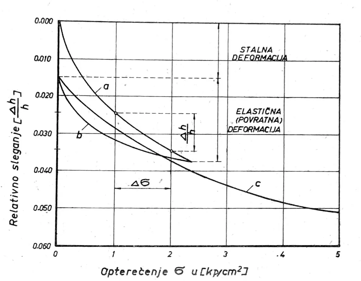
This diagram is obtained when normal pressure is applied to the sample on the abscissa axis σ = P/A, where P is the load acting on the sample via the upper filter stone in kp/cm2, A is the cross-sectional area of the sample in the apparatus, and on the ordinate axis is the relative compression Δh/h where Δh is the settlement of the sample under load Δσ during consolidation, h is the height of the sample before loading (fig. 2).

Sl. 2. Relative Compression Diagram
During loading, the diagram of primary compression a. is obtained
During unloading, if the unhindered intake of water is enabled, so that the sample remained under water during unloading, it returns to its original state, i.e. swelling. However, the sample does not return to its initial state, which means that it has undergone plastic (permanent) deformation in addition to elastic. Therefore, in this case, the swelling diagram b is obtained during unloading. However, if the test was performed without receiving water, instead of a swelling diagram, the so-called diagram of elasticity.
If the sample is loaded again after unloading, the diagram of secondary compression c is obtained. The swelling diagram and the secondary compression diagram c form a hysteresis loop between them. In clay, the hysteresis loops are significant and therefore the deformation in the area of swelling and secondary compression (diagrams b and c) are not considered elastic, but reversible, since they are not proportional to the load according to Hooke’s law. Deformations in the area of primary compression (diagram a) in the part where they did not return are permanent (irreversible).
Soil compressibility modulus
From the diagram of relative compression, we obtain according to Hooke’s law, analogously to Jung’s modulus of elasticity E for an elastic material, the compressibility modulus of the soil Ms
Ms = Δσ / (Δh/h) [kp/cm2],
where Δσ is the load increment, Δh/h is the corresponding relative compression, which is taken from the primary compression diagram a (fig. 2).
The soil compressibility modulus Ms differs from the elasticity modulus E of an elastic material, because Ms is not constant for one and the same material but is variable and increases with the normal load σ. Therefore, one specific value of compressibility modulus Ms can be given only for one narrow interval of normal soil load Δσ. If the value of the module Ms is higher, the compressibility of the soil is lower and vice versa. According to our foundation regulations, the following criterion is adopted for the compressibility modulus of the soil in its natural state:
The classification below is carried over from the original text, including the repeated interval 100-400 kp/cm2. It has not been checked or harmonized with current regulations.
Ms = 0 - 20 kp/cm2 extraordinarily compressible soil
Ms = 20 - 50 kp/cm2 very compressible soil
Ms = 50 - 100 kp/cm2 medium compressible soil
Ms = 100 - 400 kp/cm2 less compressible soil
Ms = 100 - 400 kp/cm2 slightly compressible soil
Ms = 400 - 1000 kp/cm2 slightly compressible soil
Ms > 1000 kp/cm2 very low compressible soil.
Modulus of elasticity of the soil
In the same way, we obtain the modulus of elasticity of the soil E:
E = Δσ / (Δh/h) [kp/cm2],
where the relative compression increment Δh/h is taken from the soil elasticity diagram for the corresponding normal pressure increment Δσ.
Normal consolidated and overconsolidated soil

Sl. 3. Diagram of change of porosity coefficient of disturbed soil sample
If we perform an oedometer test with a disturbed sample, which we entered into the apparatus at the yield point, and we plot the results of the test on the diagram of the change in the porosity coefficient e depending on the pressure σ (fig. 3), the consolidation flow is represented by the diagrams 1 for primary loading, 2 for unloading, 3 for the secondary load up to the limit a of the primary load extension σa and 4 beyond that limit.
The unloading diagram 2 and the secondary compression diagram 3 form a hysteresis loop behind which the diagram 4 continues in the extension of the diagram 1, without breaks, as if there was no unloading and reloading.

Sl. 4. Diagram of change of porosity coefficient of undisturbed soil sample
However, if we perform the oedometer test in the same way as before with an undisturbed sample taken from a certain depth of the soil (fig. 4), the diagram for the secondary load 3 will show, at a certain load σb, a fracture at point b, after which the diagram 4 will have a greater slope. This fracture occurred because the soil from which the sample was taken was under a greater load p=γt than the load of the sample σ in the oedometer. The higher load p originates from the weight of the existing upper soil layers to the surface of the terrain, which we call soil pressure, or from the load of earlier soil layers carried away over time by erosion or moraine soil or ice, which we call preload. The appearance of overconsolidation is particularly characteristic of clay, where we distinguish between normally consolidated and overconsolidated clay.
Normally consolidated clay
Normally consolidated clay is at shallower depths below the ground surface, which has not been previously exposed to preload. A sample of this clay, loaded in the oedometer with loads greater than the weight of the upper “soil pressure” layers, shows a continuous flow of consolidation, without breaks in the relative compression diagram or in the porosity coefficient change diagram. The settlement of this clay under the load of the object is normal, i.e. under a certain load, settlement decreases over time.
Overconsolidated clay
Overconsolidated clay is at greater depths or has previously been subjected to preloading. A sample of this clay loaded in the oedometer with a pressure greater than the soil pressure or preload shows a fracture on the relative compression diagram or on the porosity coefficient change diagram, the so-called. geological fracture g, with a strong change in direction (fig. 5a). The settlement of this clay under the structure is small for loads below soil pressure or preload σ1, but becomes significantly larger for loads above σ1.
If the geological fracture is not clearly defined, then it is determined using tangents to the diagram (Fig. 5b).

Sl. 5. Diagram of changes in porosity coefficient of overconsolidated clay
Time settlement diagram
This diagram, also called the consolidation diagram, is obtained when, for each level of load of the sample in the oedometer, the time t in hours is applied to the abscissa axis, and the settlement in mm (fig. 6a) or in % of the total settlement (fig. 6b) to the ordinate axis.

Sl. 6. Time Settlement Diagram
Unbound and bound soils behave differently under load. Loose soils, such as sand, have large pores, from which water is quickly squeezed out under load, so that the soil settles quickly, with the largest settlement occurring at the beginning of the load and reaching the final settlement at a given load in a relatively short time interval. Cohesive soils such as clay have small pores from which water is difficult to squeeze out under load. There are two phases in the time process of compacted soil settlement. In the first phase, immediately after applying the load to the soil, since the water cannot flow out of the pores, it becomes stressed and receives the entire applied load. In the second stage, the stressed pore water begins to push out under its own stress due to the load, which is gradually transferred to the solid soil particles. In this second phase, the particles come together and the pores shrink. The subsidence process continues until the pressure water is forced out of the pores, i.e. until the stressed state of water in the pores ceases to exist. Therefore, soil consolidation is primarily a hydrodynamic problem, which depends on soil permeability and porosity. In the case of clay, whose permeability is low, the consolidation process can take a very long time, and in addition, the settlements can be significantly greater due to the higher total porosity than in the case of sand. On the basis of the consolidation test, the calculation of the time course of settlement can be made for the entire duration of the consolidation and in individual phases.